2. Constructing Models
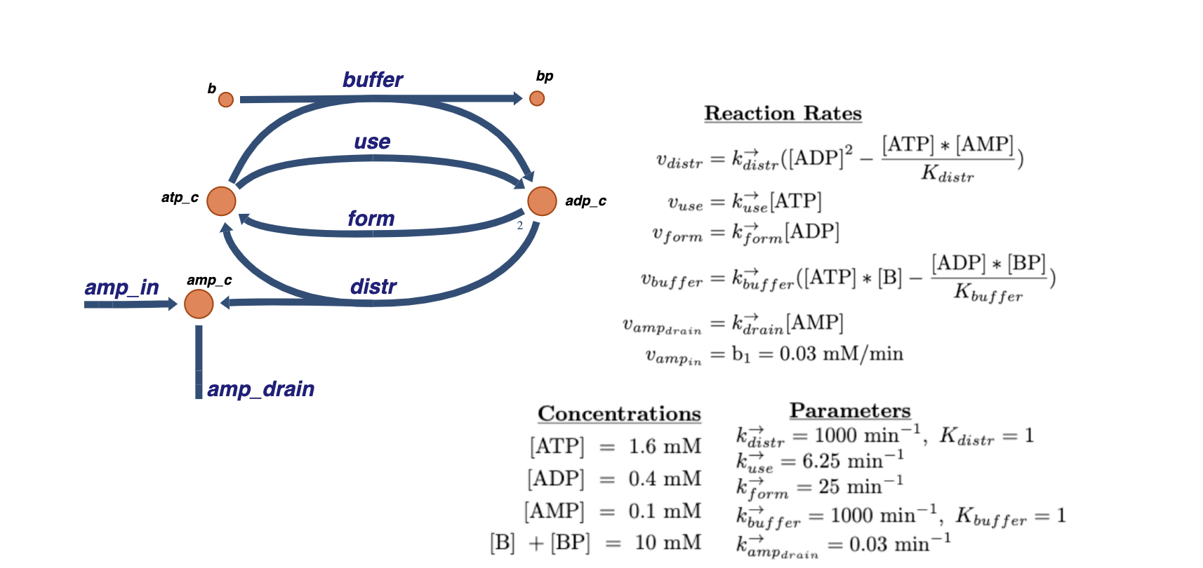
In this notebook example, a step-by-step approach of building a simple model\(^1\) of trafficking of high-energy phosphate bonds is demonstrated. Illustrated below is a graphical view of the full system along with the reaction rate equations and numerical values:
The example starts by creating a model of the “use”, “distr”, and “form” reactions. Then the model is expanded to include the remaining metabolites, reactions, and any additional information that should be defined in the model.
2.1. Creating a Model
[1]:
import numpy as np
import pandas as pd

from mass import (
    MassConfiguration, MassMetabolite, MassModel, MassReaction)
from mass.util.matrix import left_nullspace, nullspace

mass_config = MassConfiguration()
The first step to creating the model is to define the MassModel object. A MassModel only requires an identifier to be initialized. For best practice, it is recommended to utilize SBML compliant identifiers for all objects.
[2]:
model = MassModel("Phosphate_Trafficking")
Set parameter Username
The model is initially empty.
[3]:
print("Number of metabolites: {0}".format(len(model.metabolites)))
print("Number of initial conditions: {0}".format(len(model.initial_conditions)))
print("Number of reactions: {0}".format(len(model.reactions)))
Number of metabolites: 0
Number of initial conditions: 0
Number of reactions: 0
The next step is to create MassMetabolite and MassReaction objects to represent the metabolites and reactions that should exist in the model.
2.1.1. Defining metabolites
To create a MassMetabolite, a unique identifier is required. The formula and charge attributes are set to ensure mass and charge balancing of reactions in which the metabolite is a participant. The compartment attribute indicates where the metabolite is located. In this model, all metabolites exist in a single compartment, abbreviated as “c”.
[4]:
atp_c = MassMetabolite(
    "atp_c",
    name="ATP",
    formula="C10H12N5O13P3",
    charge=-4,
    compartment="c")

adp_c = MassMetabolite(
    "adp_c",
    name="ADP",
    formula="C10H12N5O10P2",
    charge=-3,
    compartment="c")

amp_c = MassMetabolite(
    "amp_c",
    name="AMP",
    formula="C10H12N5O7P",
    charge=-2,
    compartment="c")
The metabolite concentrations can be defined as the initial conditions for the metabolites using the initial_condition attribute. As previously stated, the concentrations are \(\text{[ATP]}=1.6\), \(\text{[ADP]}=0.4\), and \(\text{[AMP]}=0.1\).
[5]:
atp_c.initial_condition = 1.6
adp_c.ic = 0.4  # Alias for initial_condition
amp_c.ic = 0.1

for metabolite in [atp_c, adp_c, amp_c]:
    print("{0}: {1}".format(metabolite.id, metabolite.initial_condition))
atp_c: 1.6
adp_c: 0.4
amp_c: 0.1
The metabolites are currently not a part of any reaction. Consequently, the ordinary_differential_equation attribute is None.
[6]:
print(atp_c.ordinary_differential_equation)
print(adp_c.ode)  # Alias for ordinary_differential_equation
print(amp_c.ode)
None
None
None
The next step is to create the reactions in which the metabolites participate.
2.1.2. Defining reactions
Just like MassMetabolite objects, a unique identifier is also required to create a MassReaction. The reversible attribute determines whether the reaction can proceed in both the forward and reverse directions, or only in the forward direction.
[7]:
distr = MassReaction("distr", name="Distribution", reversible=True)
use = MassReaction("use", name="ATP Utilization", reversible=False)
form = MassReaction("form", name="ATP Formation", reversible=False)
Metabolites are added to reactions using a dictionary of metabolite objects and their stoichiometric coefficients. A group of metabolites can be added either all at once or one at a time. A negative coefficient indicates the metabolite is a reactant, while a positive coefficient indicates the metabolite is a product.
[8]:
distr.add_metabolites({
    adp_c: -2,
    atp_c: 1,
    amp_c: 1})

use.add_metabolites({
    atp_c: -1,
    adp_c: 1})

form.add_metabolites({
    adp_c: -1,
    atp_c: 1})

for reaction in [distr, use, form]:
    print(reaction)
distr: 2 adp_c <=> amp_c + atp_c
use: atp_c --> adp_c
form: adp_c --> atp_c
Once the reactions are created, their parameters can be defined. As stated earlier, the distribution reaction is considerably faster when compared to other reactions in the model. The forward rate constant \(k^{\rightarrow}\), represented as kf, can be set as \(k^{\rightarrow}_{distr}=1000\ \text{min}^{-1}\). The equilibrium constant \(K_{eq}\), represented as Keq, is approximately \(K_{distr}=1\).
[9]:
distr.forward_rate_constant = 1000
distr.equilibrium_constant = 1
distr.parameters  # Return defined mass action kinetic parameters
[9]:
{'kf_distr': 1000, 'Keq_distr': 1}
As shown earlier, the forward rate constants are set as \(k^{\rightarrow}_{use}=6.25\ \text{min}^{-1}\) and \(k^{\rightarrow}_{form}=25\ \text{min}^{-1}\). The kf_str attribute can be used to get the identifier of the forward rate constant as a string.
[10]:
use.forward_rate_constant = 6.25
form.kf = 25  # Alias for forward_rate_constant

print("{0}: {1}".format(use.kf_str, use.kf))
print("{0}: {1}".format(form.kf_str, form.kf))
kf_use: 6.25
kf_form: 25
Reactions can be added to the model using the add_reactions() method. Adding the reactions to the model also adds the associated metabolites and genes.
[11]:
model.add_reactions([distr, use, form])

print("Number of metabolites: {0}".format(len(model.metabolites)))
print("Number of initial conditions: {0}".format(len(model.initial_conditions)))
print("Number of reactions: {0}".format(len(model.reactions)))
Number of metabolites: 3
Number of initial conditions: 3
Number of reactions: 3
The stoichiometric matrix of the model is automatically constructed with the addition of the reactions and metabolites to the model. It can be accessed through the stoichiometric_matrix property (alias S).
[12]:
print(model.S)
[[-2.  1. -1.]
 [ 1. -1.  1.]
 [ 1.  0.  0.]]
The stoichiometric matrix attribute can be updated and stored in various formats using the update_S() method. For example, the stoichiometric matrix can be converted and stored as a pandas.DataFrame.
[13]:
model.update_S(array_type="DataFrame", dtype=np.int_, update_model=True)
model.S
[13]:
| distr | use | form | |
|---|---|---|---|
| adp_c | -2 | 1 | -1 |
| atp_c | 1 | -1 | 1 |
| amp_c | 1 | 0 | 0 |
Associating the metabolites with reactions allows for the mass action reaction rate expressions to be generated based on the stoichiometry.
[14]:
print(distr.rate)
kf_distr*(adp_c(t)**2 - amp_c(t)*atp_c(t)/Keq_distr)
Generation of the reaction rates also allows for the metabolite ODEs to be generated.
[15]:
print(atp_c.ode)
kf_distr*(adp_c(t)**2 - amp_c(t)*atp_c(t)/Keq_distr) + kf_form*adp_c(t) - kf_use*atp_c(t)
The nullspace() method can be used to obtain the null space of the stoichiometric matrix. The nullspace reflects the pathways through the system.
[16]:
ns = nullspace(model.S)  # Get the null space
# Divide by the minimum and round to nearest integer
ns = np.rint(ns / np.min(ns[np.nonzero(ns)]))
pd.DataFrame(
    ns, index=model.reactions.list_attr("id"),  # Rows represent reactions
    columns=["Pathway 1"], dtype=np.int_)
[16]:
| Pathway 1 | |
|---|---|
| distr | 0 |
| use | 1 |
| form | 1 |
In a similar fashion the left nullspace can be obtained using the left_nullspace function. The left nullspace represents the conserved moieties in the model.
[17]:
lns = left_nullspace(model.S)
# Divide by the minimum and round to nearest integer
lns = np.rint(lns / np.min(lns[np.nonzero(lns)]))
pd.DataFrame(
    lns, index=["Total AxP"],
    columns=model.metabolites.list_attr("id"),  # Columns represent metabolites
    dtype=np.int_)
[17]:
| adp_c | atp_c | amp_c | |
|---|---|---|---|
| Total AxP | 1 | 1 | 1 |
2.2. Expanding an Existing Model
Now, the existing model is expanded to include a buffer reaction, where a phosphagen is utilized to store a high-energy phosphate in order to buffer the ATP/ADP ratio as needed. Because the buffer molecule represents a generic phosphagen, there is no chemical formula for the molecule. Therefore, the buffer molecule can be represented as a moiety in the formula attribute using square brackets.
[18]:
b = MassMetabolite(
    "B",
    name="Phosphagen buffer (Free)",
    formula="[B]",
    charge=0,
    compartment="c")

bp = MassMetabolite(
    "BP",
    name="Phosphagen buffer (Loaded)",
    formula="[B]-PO3",
    charge=-1,
    compartment="c")

buffer = MassReaction("buffer", name="ATP Buffering")
When adding metabolites to the reaction, the get_by_id() method is used to add already existing metabolites in the model to the reaction.
[19]:
buffer.add_metabolites({
    b: -1,
    model.metabolites.get_by_id("atp_c"): -1,
    model.metabolites.get_by_id("adp_c"): 1,
    bp: 1})

# Add reaction to model
model.add_reactions([buffer])
For this reaction, \(k^{\rightarrow}_{buffer}=1000\ \text{min}^{-1}\) and \(K_{buffer}=1\). Because the reaction has already been added to the model, the MassModel.update_parameters() method can be used to update the reaction parameters using a dictionary:
[20]:
model.update_parameters({
    buffer.kf_str: 1000,
    buffer.Keq_str: 1})

buffer.parameters
[20]:
{'kf_buffer': 1000, 'Keq_buffer': 1}
By adding the reaction to the model, the left nullspace expanded to include a conservation pool for the total buffer in the system.
[21]:
lns = left_nullspace(model.S)
for i, row in enumerate(lns):
    # Divide by the minimum and round to nearest integer
    lns[i] = np.rint(row / np.min(row[np.nonzero(row)]))
pd.DataFrame(lns, index=["Total AxP", "Total Buffer"],
             columns=model.metabolites.list_attr("id"),
             dtype=np.int_)
[21]:
| adp_c | atp_c | amp_c | B | BP | |
|---|---|---|---|---|---|
| Total AxP | 1 | 1 | 1 | 0 | 0 |
| Total Buffer | 0 | 0 | 0 | 1 | 1 |
2.2.1. Performing symbolic calculations
Although the concentrations for the free and loaded buffer molecules are currently unknown, the total amount of buffer is known and set as \(B_{total} = 10\). Because the buffer reaction is assumed to be at equilibrium, it becomes possible to solve for the concentrations of the free and loaded buffer molecules.
Below, the symbolic capabilities of SymPy are used to solve for the steady state concentrations of the buffer molecules.
[22]:
from sympy import Eq, Symbol, pprint, solve

from mass.util import strip_time
The first step is to define the equation for the total buffer pool symbolically:
[23]:
buffer_total_equation = Eq(Symbol("B") + Symbol("BP"), 10)
pprint(buffer_total_equation)
B + BP = 10
The equation for the reaction rate at equilibrium is also defined. The strip_time() function is used to strip time dependency from the equation.
[24]:
buffer_rate_equation = Eq(0, strip_time(buffer.rate))
# Substitute defined concentration values into equation
buffer_rate_equation = buffer_rate_equation.subs({
    "atp_c":  atp_c.initial_condition,
    "adp_c":  adp_c.initial_condition,
    "kf_buffer": buffer.kf,
    "Keq_buffer": buffer.Keq})
pprint(buffer_rate_equation)
0 = 1600.0⋅B - 400.0⋅BP
These two equations can be solved to get the buffer concentrations:
[25]:
buffer_sol = solve([buffer_total_equation, buffer_rate_equation],
                   [Symbol("B"), Symbol("BP")])
buffer_sol
[25]:
{B: 2.00000000000000, BP: 8.00000000000000}
Because the metabolites already exist in the model, their initial conditions can be updated to the calculated concentrations using the MassModel.update_initial_conditions() method.
[26]:
# Replace the symbols in the dict
for met_symbol, concentration in buffer_sol.copy().items():
    metabolite = model.metabolites.get_by_id(str(met_symbol))
    # Make value as a float
    buffer_sol[metabolite] = float(buffer_sol.pop(met_symbol))

model.update_initial_conditions(buffer_sol)
model.initial_conditions
[26]:
{<MassMetabolite adp_c at 0x7f8368c373a0>: 0.4,
 <MassMetabolite atp_c at 0x7f8368c377c0>: 1.6,
 <MassMetabolite amp_c at 0x7f8368c37f70>: 0.1,
 <MassMetabolite B at 0x7f8359672160>: 2.0,
 <MassMetabolite BP at 0x7f8359672b50>: 8.0}
2.2.2. Adding boundary reactions
After adding the buffer reactions, the next step is to define the AMP source and demand reactions. The add_boundary() method is employed to create and add a boundary reaction to a model.
[27]:
amp_drain = model.add_boundary(
    model.metabolites.amp_c,
    boundary_type="demand",
    reaction_id="amp_drain")

amp_in = model.add_boundary(
    model.metabolites.amp_c,
    boundary_type="demand",
    reaction_id="amp_in")

print(amp_drain)
print(amp_in)
amp_drain: amp_c -->
amp_in: amp_c -->
When a boundary reaction is created, a ‘boundary metabolite’ is also created as a proxy metabolite. The proxy metabolite is the external metabolite concentration (i.e., boundary condition) without instantiating a new MassMetabolite object to represent the external metabolite.
[28]:
amp_in.boundary_metabolite
[28]:
'amp_b'
The value of the ‘boundary metabolite’ can be set using the MassModel.add_boundary_conditions() method. Boundary conditions are accessed through the MassModel.boundary_conditions attribute.
[29]:
model.add_boundary_conditions({amp_in.boundary_metabolite: 1})
model.boundary_conditions
[29]:
{'amp_b': 1.0}
The automatic generation of the boundary reaction can be useful. However, sometimes the reaction stoichiometry needs to be switched in order to be intuitive. In this case, the stoichiometry of the AMP source reaction should be reversed to show that AMP enters the system, which is accomplished by using the MassReaction.reverse_stoichiometry() method.
[30]:
amp_in.reverse_stoichiometry(inplace=True)
print(amp_in)
amp_in: --> amp_c
Note that the addition of these two reactions adds an another pathway to the null space:
[31]:
ns = nullspace(model.S).T
for i, row in enumerate(ns):
    # Divide by the minimum to get all integers
    ns[i] = np.rint(row / np.min(row[np.nonzero(row)]))
ns = ns.T
pd.DataFrame(
    ns, index=model.reactions.list_attr("id"),  # Rows represent reactions
    columns=["Path 1", "Path 2"], dtype=np.int_)
[31]:
| Path 1 | Path 2 | |
|---|---|---|
| distr | 0 | 0 |
| use | 1 | 0 |
| form | 1 | 0 |
| buffer | 0 | 0 |
| amp_drain | 0 | 1 |
| amp_in | 0 | 1 |
2.2.3. Defining custom rates
In this model, the rate for the AMP source reaction should remain at a fixed input value. However, the current rate expression for the AMP source reaction is dependent on an external AMP metabolite that exists as a boundary condition:
[32]:
print(amp_in.rate)
amp_b*kf_amp_in
Therefore, the rate can be set as a fixed input by using a custom rate expression. Custom rate expressions can be set for reactions in a model using the MassModel.add_custom_rate() method as follows: by passing the reaction object, a string representation of the custom rate expression, and a dictionary containing any custom parameter associated with the rate.
[33]:
model.add_custom_rate(amp_in, custom_rate="b1",
                      custom_parameters={"b1": 0.03})
print(model.rates[amp_in])
b1
2.3. Ensuring Model Completeness
2.3.1. Inspecting rates and ODEs
According to the network schema at the start of the notebook, the network has been fully reconstructed. The reaction rates and metabolite ODEs can be inspected to ensure that the model was built without any issues.
The MassModel.rates property is used to return a dictionary containing reactions and symbolic expressions of their rates. The model always prioritizes custom rate expressions over automatically generated mass action rates.
[34]:
for reaction, rate in model.rates.items():
    print("{0}: {1}".format(reaction.id, rate))
distr: kf_distr*(adp_c(t)**2 - amp_c(t)*atp_c(t)/Keq_distr)
use: kf_use*atp_c(t)
form: kf_form*adp_c(t)
buffer: kf_buffer*(B(t)*atp_c(t) - BP(t)*adp_c(t)/Keq_buffer)
amp_drain: kf_amp_drain*amp_c(t)
amp_in: b1
Similarly, the model can access the ODEs for metabolites using the ordinary_differential_equations property (alias odes) to return a dictionary of metabolites and symbolic expressions of their ODEs.
[35]:
for metabolite, ode in model.odes.items():
    print("{0}: {1}".format(metabolite.id, ode))
adp_c: kf_buffer*(B(t)*atp_c(t) - BP(t)*adp_c(t)/Keq_buffer) - 2*kf_distr*(adp_c(t)**2 - amp_c(t)*atp_c(t)/Keq_distr) - kf_form*adp_c(t) + kf_use*atp_c(t)
atp_c: -kf_buffer*(B(t)*atp_c(t) - BP(t)*adp_c(t)/Keq_buffer) + kf_distr*(adp_c(t)**2 - amp_c(t)*atp_c(t)/Keq_distr) + kf_form*adp_c(t) - kf_use*atp_c(t)
amp_c: b1 - kf_amp_drain*amp_c(t) + kf_distr*(adp_c(t)**2 - amp_c(t)*atp_c(t)/Keq_distr)
B: -kf_buffer*(B(t)*atp_c(t) - BP(t)*adp_c(t)/Keq_buffer)
BP: kf_buffer*(B(t)*atp_c(t) - BP(t)*adp_c(t)/Keq_buffer)
2.3.2. Compartments
Compartments, defined in metabolites, are recognized by the model and can be viewed in the compartments attribute.
[36]:
model.compartments
[36]:
{'c': ''}
For this model, “c” is an abbreviation for “compartment”. The compartments attribute can be updated to reflect this mapping using a dict:
[37]:
model.compartments = {"c": "compartment"}
model.compartments
[37]:
{'c': 'compartment'}
2.3.3. Units
Unit and UnitDefinition objects are implemented as per the SBML Unit and SBML UnitDefinition specifications. It can be useful for comparative reasons to create Unit and UnitDefinition objects for the model (e.g., amount, volume, time) to provide
additional context. However, the model does not maintain unit consistency automatically. It is the responsibility of the users to ensure consistency among units and associated numerical values in a model.
[38]:
from mass import Unit, UnitDefinition
from mass.core.units import print_defined_unit_values
SBML defines units using a compositional approach. The Unit objects represent references to base units. A Unit has four attributes: kind, exponent, scale, and multiplier. The kind attribute indicates the base unit. Valid base units are viewed using the print_defined_unit_values() function.
[39]:
print_defined_unit_values("BaseUnitKinds")
╒═════════════════════════════╕
│ SBML Base Unit Kinds        │
╞═════════════════════════════╡
│ Base Unit        SBML Value │
│ -------------  ------------ │
│ ampere                    0 │
│ avogadro                  1 │
│ becquerel                 2 │
│ candela                   3 │
│ coulomb                   5 │
│ dimensionless             6 │
│ farad                     7 │
│ gram                      8 │
│ gray                      9 │
│ henry                    10 │
│ hertz                    11 │
│ item                     12 │
│ joule                    13 │
│ katal                    14 │
│ kelvin                   15 │
│ kilogram                 16 │
│ liter                    17 │
│ litre                    18 │
│ lumen                    19 │
│ lux                      20 │
│ meter                    21 │
│ metre                    22 │
│ mole                     23 │
│ newton                   24 │
│ ohm                      25 │
│ pascal                   26 │
│ radian                   27 │
│ second                   28 │
│ siemens                  29 │
│ sievert                  30 │
│ steradian                31 │
│ tesla                    32 │
│ volt                     33 │
│ watt                     34 │
│ weber                    35 │
│ invalid                  36 │
╘═════════════════════════════╛
The exponent, scale and multiplier attributes indicate how the base unit should be transformed. For this model, the unit for concentration, “Millimolar”, which is represented as millimole per liter and composed of the following base units:
[40]:
millimole = Unit(kind="mole", exponent=1, scale=-3, multiplier=1)
per_liter = Unit(kind="liter", exponent=-1, scale=1, multiplier=1)
Combinations of Unit objects are contained inside a UnitDefintion object. UnitDefinition objects have three attributes: an id, an optional name to represent the combination, and a list_of_units attribute that contain references to the Unit objects. The concentration unit “Millimolar” is abbreviated as “mM” and defined as follows:
[41]:
concentration_unit = UnitDefinition(id="mM", name="Millimolar",
                                    list_of_units=[millimole, per_liter])
print("{0}:\n{1!r}\n{2!r}".format(
    concentration_unit.name, *concentration_unit.list_of_units))
Millimolar:
<Unit at 0x7f835967d1c0 kind: mole; exponent: 1; scale: -3; multiplier: 1>
<Unit at 0x7f835967dbe0 kind: liter; exponent: -1; scale: 1; multiplier: 1>
UnitDefinition objects also have the UnitDefinition.create_unit() method to directly create Unit objects within the UnitDefintion.
[42]:
time_unit = UnitDefinition(id="min", name="Minute")
time_unit.create_unit(kind="second", exponent=1, scale=1, multiplier=60)
print(time_unit)
print(time_unit.list_of_units)
min
[<Unit at 0x7f8309bbea90 kind: second; exponent: 1; scale: 1; multiplier: 60>]
Once created, UnitDefintion objects are added to the model:
[43]:
model.add_units([concentration_unit, time_unit])
model.units
[43]:
[<UnitDefinition Millimolar "mM" at 0x7f8318e6b970>,
 <UnitDefinition Minute "min" at 0x7f8309bbe8b0>]
2.3.4. Checking model completeness
Once constructed, the model should be checked for completeness.
[44]:
from mass import qcqa_model
The qcqa_model() function can be used to print a report about the model’s completeness based on the set kwargs. The qcqa_model() function is used to ensure that all numerical values necessary for simulating the model are defined by setting the parameters and concentrations kwargs as True.
[45]:
qcqa_model(model, parameters=True, concentrations=True)
╒══════════════════════════════════════════════╕
│ MODEL ID: Phosphate_Trafficking              │
│ SIMULATABLE: False                           │
│ PARAMETERS NUMERICALY CONSISTENT: True       │
╞══════════════════════════════════════════════╡
│ ============================================ │
│             MISSING PARAMETERS               │
│ ============================================ │
│ Reaction Parameters                          │
│ ---------------------                        │
│ amp_drain: kf                                │
│ ============================================ │
╘══════════════════════════════════════════════╛
As shown in the report above, the forward rate constant for the AMP drain reaction was never defined. Therefore, the forward rate constant is defined, and the model is checked again.
[46]:
amp_drain.kf = 0.03

qcqa_model(model, parameters=True, concentrations=True)
╒══════════════════════════════════════════╕
│ MODEL ID: Phosphate_Trafficking          │
│ SIMULATABLE: True                        │
│ PARAMETERS NUMERICALY CONSISTENT: True   │
╞══════════════════════════════════════════╡
╘══════════════════════════════════════════╛
Now, the report shows that the model is not missing any values necessary for simulation. See Checking Model Quality for more information on quality assurance functions and the qcqa submodule.
2.4. Additional Examples
For additional examples on constructing models, see the following:
\(^1\) Trafficking model is created from Chapter 8 of [Pal11]