7. Orders of Magnitude
The simulation examples in the previous chapters are conceptual. As we begin to build simulation models of realistic biological processes, the need to obtain information such as the numerical values of the parameters that appear in the dynamic mass balances. We thus go through a process of estimating the approximate numerical values of various quantities and parameters. Size, mass, chemical composition, metabolic complexity, and genetic makeup represent characteristics for which we now have extensive data available. Based on typical values for these quantities we show how one can make useful estimates of concentrations and the dynamic features of the intracellular environment.
7.1. Cellular Composition and Ultra-structure
It is often stated that all biologists have two favorite organisms, E. coli and another one. Fortunately, much data exists for E. coli, and we can go through parameter and variable estimation procedures using it as an example. These estimation procedures can be performed for other target organisms, cell types, and cellular processes in an analogous manner if the appropriate data is available. We organize the discussion around key questions.
7.1.1. The interior of a cell
The typical bacterial cell, like E. coli, is on the order of microns in size (Figure 7.1a). The E. coli cell is a short cylinder, about 2-4 micron in length with a 0.5 to 1.5 micron diameter, Figure 7.1b. The size of the E. coli cell is growth rate dependent; the faster the cell grows, the larger it is.
It has a complex intra-cellular environment. One can isolate and crystallize macromolecules and obtain their individual structure. However, this approach gives limited information about the configuration and location of a protein in a living functional cell. The intracellular milieu can to be reconstructed from available data to yield an indirect picture of the interior of an cell. Such a reconstruction has been carried out Goodsell93. Based on well known chemical composition data, this image provides us with about a million-fold magnification of the interior of an E. coli cell, see Figure 7.1c. Examination of this picture of the interior of the E. coli cell is instructive:
The intracellular environment is very crowded and represents a dense solution. Protein density in some sub-cellular structures can approach that found in protein crystals, and the intracellular environment is sometimes referred to as ‘soft glass,’ suggesting that it is close to a crystalline state.
The chemical composition of this dense mixture is very complex. The majority of cellular mass are macromolecules with metabolites, the small molecular weight molecules interspersed among the macromolecules.
In this crowded solution, the motion of the macromolecules is estimated to be one hundred to even one thousand-fold slower than in a dilute solution. The time it takes a 160 kDa protein to move 10 nm - a distance that corresponds approximately to the size of the protein molecule - is estimated to be 0.2 to 2 milliseconds. Moving one cellular diameter of approximately 0.64 \(\mu m\), or 640 nm, would then require 1-10 min. The motion of metabolites is expected to be significantly faster due to their smaller size.
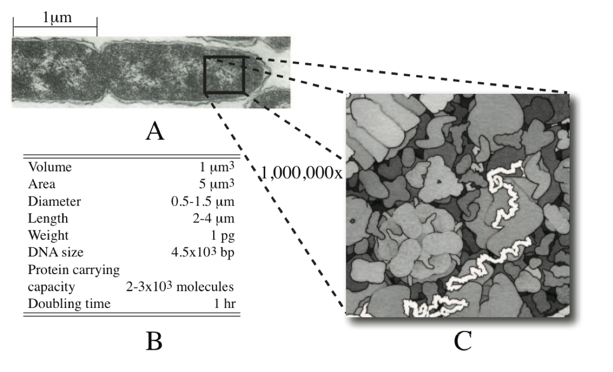
Figure 7.1: (a) An electron micrograph of the E. coli cell, from Ingraham83. (b) Characteristic features of an E. coli cell. (c) The interior of an E. coli cell, © David S. Goodsell 1999.
7.1.2. The overall chemical composition of a cell
With these initial observations, let’s take a closer look at the chemical composition of the cell. Most cells are about 70% water. It is likely that cellular functions and evolutionary design is constrained by the solvent capacity of water, and the fact that most cells are approximately 70% water suggests that all cells are close to these constraints.
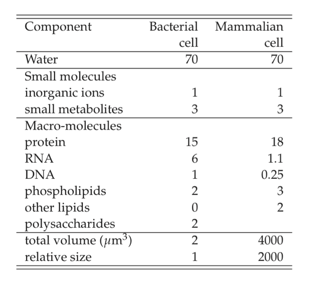
The ‘biomass’ is about 30% of cell weight. It is sometimes referred to as the dry weight of a cell, and is denoted by gDW. The 30% of the weight that is biomass is comprised of 26% macromolecules, 1% inorganic ions, and 3% low molecular weight metabolites. The basic chemical makeup of prokaryotic cells is shown in Table 7.1, and contrasted to that of a typical animal cell. The gross chemical composition is similar except that animal cells, and eukaryotic cells in general, have a higher lipid content because of the membrane requirement for cellular compartmentalization. Approximate cellular composition is available or relatively easy to get for other cell types.
Table 7.1: Approximate composition of cells, from (Alberts, 1983). The numbers given are weight percent.
7.1.3. The detailed composition of E. coli
The total weight of a bacterial cell is about 1 picogram. The density of cells barely exceeds that of water, and cellular density is typically around 1.04 to 1.08 \(gm/cm^3\). Since the density of cells is close to unity, a cellular concentration of about \(10^12\) cells per milliliter represents packing density of E. coli cells. Detailed and recent data is found later in Figure 7.2.
This information provides the basis for estimating the numerical values for a number of important quantities that relate to dynamic network modeling. Having such order of magnitude information provides a frame of reference, allows one to develop a conceptual model of cells, evaluate the numerical outputs from models, and perform any approximation or simplification that is useful and justified based on the numbers. “Numbers count,” even in biology.
7.1.4. Order of magnitude estimates
It is relatively easy to estimate the approximate order of magnitude of the numerical values of key quantities. Enrico Fermi the famous physicist was well-known for his skills with such calculations and they thus know as Fermi problems. We give a couple examples to illustrate the order of magnitude estimation process.
7.1.4.1. 1. How many piano tuners are in Chicago?
This question represents a classical Fermi problem. First we state assumptions or key numbers:
1. There are approximately 5,000,000 people living in Chicago.
2. On average, there are two persons in each household in Chicago.
3. Roughly one household in twenty has a piano that is tuned regularly.
4. Pianos that are tuned regularly are tuned on average about once per year.
5. It takes a piano tuner about two hours to tune a piano, including travel time.
6. Each piano tuner works eight hours in a day, five days in a week, and 50 weeks in a year.
From these assumptions we can compute:
that the number of piano tunings in a single year in Chicago is: (5,000,000 persons in Chicago)/(2 persons/household) \(*\) (1 piano/20 households) \(*\) (1 piano tuning per piano per year) = 125,000 piano tunings per year in Chicago.
that the average piano tuner performs (50 weeks/year) \(*\) (5 days/week) \(*\) (8 hours/day)/(1 piano tuning per 2 hours per piano tuner) = 1000 piano tunings per year per piano tuner.
then dividing gives (125,000 piano tuning per year in Chicago) / (1000 piano tunings per year per piano tuner) = 125 piano tuners in Chicago, which is the answer that we sought.
7.1.4.2. 2. How far can a retrovirus diffuse before it falls apart?
A similar procedure that relies more on scientific principles can be used to answer this question. The half-live of retroviruses, \(t_{0.5}\), are measured to be about 5 to 6 hours. The time constant for diffusion is:
where l is the diffusion distance and \(D\) is the diffusion constant. Then the distance \(l_{0.5}\) that a virus can travel over a half life is
Using a numerical value for \(D\) of \(6.5*10^{-8}\ cm^2/sec\) that is computed from the Stokes-Einstein equation for a 100 nm particle (approximately the diameter of the retrovirus) the estimate is about 500 \(\mu m\) (Chuck, 1996). A fairly short distance that limits how far a virus can go to infect a target cell.
7.1.5. A multi-scale view
The cellular composition of cells is complex. More complex yet is the intricate and coordinated web of complex functions that underlie the physiological state of a cell. We can view this as a multi-scale relationship, Figure 7.2. Based on cellular composition and other data we can estimate the overall parameters that are associated with cellular functions. Here we will focus on metabolism, macro-molecular synthesis and overall cellular states.
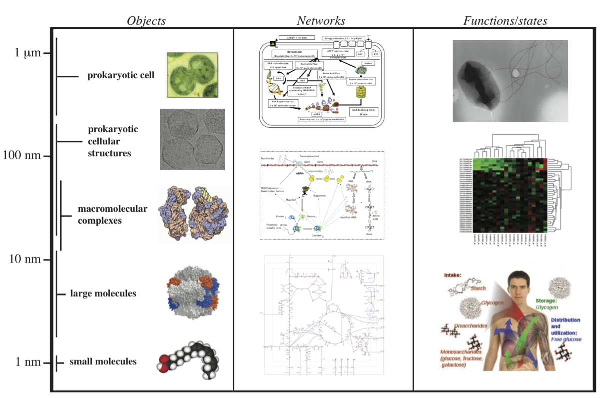
Figure 7.2: A multi-scale view of metabolism, macromolecular synthesis, and cellular functions. Prokaryotic cell (Synechocytis image from W. Vermaas, Arizona State University). Prokaryotic cell structures (purified carboxysomes) image from T. Yates, M. Yeager, and K. Dryden. Macromolecular complexes image © 2000, David S. Goodsell.
7.2. Metabolism
Biomass composition allows the estimation of important overall features of metabolic processes. These quantities are basically concentrations (abundance), rates of change (fluxes), and time constants (response times, sensitivities, etc). For metabolism, we can readily estimate reasonable values for these quantities, and we again organize the discussion around key questions.
7.2.1. What are typical concentrations?
7.2.1.1. Estimation
The approximate number of different metabolites present in a given cell is on the order of 1000 (Feist, 2007). By assuming that metabolite has a median molecular weight of about 312 gm/mol (Figure 7.3a) and that the fraction of metabolites of the wet weight is 0.01, we can estimate a typical metabolite concentration of:
The volume of a bacterial cell is about one cubic micron, or about one femto-liter \((=(10^-15)\) liter). Since a cubic micron is a logical reference volume, we convert the concentration unit as follows:
This number is remarkably small. A typical metabolite concentration of \(32 \mu M\) then translates into mere \(19,000\) molecules per cubic micron. One would expect that such low concentrations would lead to slow reaction rates. However, metabolic reaction rates are fairly rapid. As discussed in Chapter 5, cells have evolved highly efficient enzymes to achieve high reaction rates that occur even in the presence of low metabolite concentrations.
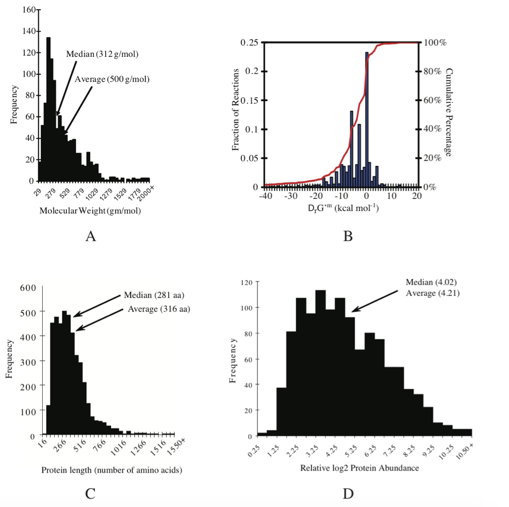
Figure 7.3: Details of E. coli K12 MG1655 composition and properties. (a) The average molecular weight of metabolites is 500 gm/mol and the median is 312 gm/mol. Molecular weight distribution. (b) Thermodynamic properties of the reactions in the iAF1260 reconstruction the metabolic network. (c) Size distribution of ORF lengths or protein sizes: protein size distribution. The average protein length is 316 amino acids, the median is 281. Average molecular weight of E. coli’s proteins (monomers): 34.7 kDa Median: 30.828 kDa (d) distribution of protein concentrations: relative protein abundance distribution. See (Feist, 2007) and (Riley, 2006) for details. Prepared by Vasiliy Portnoy.
7.2.1.2. Measurement
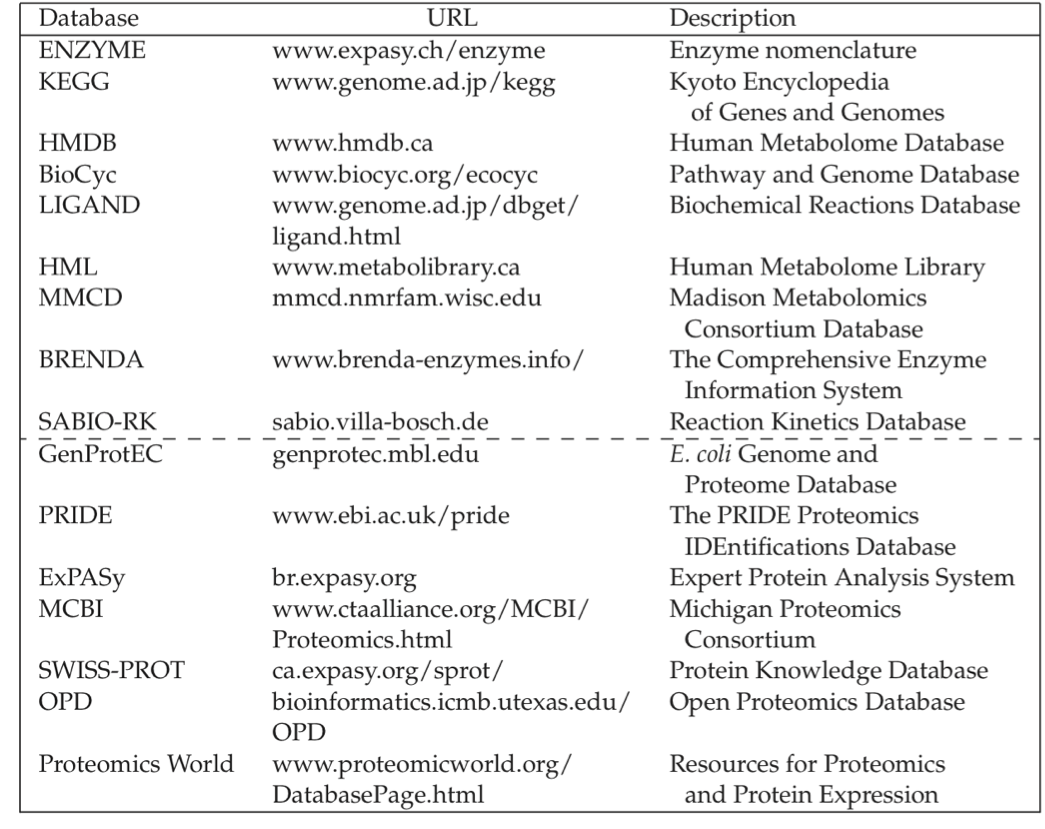
Experimentally determined ranges of metabolite concentrations fall around the estimated range; an example is provided in Table 7.2. Surprisingly, glutamate is at a concentration that falls within the 100 millimolar range in E. coli. Other important metabolites such as ATP tend to fall in the millimolar range. Intermediates of pathways are often in the micromolar range. Several on-line resources are now available for metabolic concentration data, Table 7.3.
Table 7.2: Measured and predicted parameters for E. coli growing on minimal media. Taken from (Yuan, 2006).
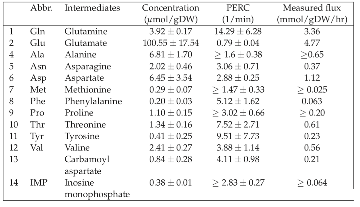
Table 7.3: Publicly available metabolic resources (above the dashed line) and proteomic resources (below the dashed line). Assembled by Vasiliy Portnoy.
7.2.2. What are typical metabolic fluxes?
7.2.2.1. Rates of diffusion
In estimating reaction rates we first need to know if they are diffusion limited. Typical cellular dimensions are on the order of microns, or less. The diffusion constants for metabolites is on the order of \(10^{-5}\ cm^2/sec\) and \(10^{-6}\ cm^2/sec\). These figures translate into diffusional response times that are on the order of:
or faster. The metabolic dynamics of interest are much slower than milliseconds. Although more detail about the cell’s finer spatial structure is becoming increasingly available, it is unlikely, from a dynamic modeling standpoint, that spatial concentration gradients will be a key concern for dynamic modeling of metabolic states in bacterial cells (Weisz, 1973).
7.2.2.2. Estimating maximal reaction rates
Reaction rates in cells are limited by the achievable kinetics. Few collections of enzyme kinetic parameters are available in the literature, see Table 7.3. One observation from such collections is that the biomolecular association rate constant, \(k_1\), for a substrate \((S)\) to an enzyme \((E)\);
is on the order of \(10^8 M^{-1} sec^{-1}\). This numerical value corresponds to the estimated theoretical limit, due to diffusional constraints (Gutfreund, 1972). The corresponding number for macromolecules is about three orders of magnitude lower.
Using the order of magnitude values for concentrations of metabolites given above and for enzymes in the next section, we find the representative association rate of substrate to enzymes to be on the order of
that translates into about
that is only one million molecules per cubic micron per second. However, the binding of the substrate to the enzyme is typically reversible and a better order of magnitude estimate for net reaction rates is obtained by considering the release rate of the product from the substrate-enzyme complex, \(X\). This release step tends to be the slowest step in enzyme catalysis (Albery 1976, Albery 1977, Cleland 1975). Typical values for the release rate constant, \(k_2\),
are \(100-1000\ sec^{-1}\). If the concentration of the intermediate substrate-enzyme complex, \(X\), is on the order of 1 \(\mu M\) we get a release rate of about
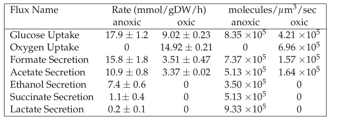
We can compare the estimate in Eq. (7.9) to observed metabolic fluxes, see Table 7.4. Uptake and secretion rates of major metabolites during bacterial growth represent high flux pathways.
Table 7.4: Typical metabolic fluxes measured in E. coli K12 MG1655 grown under oxic and anoxic conditions.
7.2.2.3. Measured kinetic constants
There are now several accessible sources of information that contain kinetic data for enzymes and the chemical transformation that they catalyze. For kinetic information, both BRENDA and SABIO-RK (Wittig, 2006) are resources of literature curated constants, including rates and saturation levels, Table 7.2.2. Unlike stoichiometric information which is universal, kinetic parameters are highly condition-dependent. In vitro kinetic assays typically do not represent in vivo conditions. Factors such as cofactor binding, pH, and unknown interactions with metabolites and proteins are likely causes.
7.2.2.4. Thermodynamics
While computational prediction of enzyme kinetic rates is difficult, obtaining thermodynamic values is more feasible. Estimates of metabolite standard transformed Gibbs energy of formation can be derived using an approach called group contribution method (Mavrovouniotis 1991). This method considers a single compound as being made up of smaller structural subgroups. The metabolite standard Gibbs energy of formation associated with structural subgroups commonly found in metabolites are available in the literature and in the NIST database urlnist. To estimate the metabolite standard Gibbs energy of formation of the entire compound, the contributions from each of the subgroups are summed along with an origin term. The group contribution approach has been used to estimate standard transformed Gibbs energy of formation for 84% of the metabolites in the genome scale model of E. coli (Feist 2007, Henry 2006, Henry 2007).
Thermodynamic values can also be obtained by integrating experimentally measured parameters and algorithms which implement sophisticated theory from biophysical chemistry (Alberty 2003, Alberty 2006). Combining this information with the results from group contribution method provides standard transformed Gibbs energy of formation for 96% of the reactions in the genome-scale E. coli model (Feist 2007), see Figure 7.3b.
7.2.3. What are typical turnover times?
As outlined in Chapter 2, turnover times can be estimated by taking that ratio of the concentration relative to the flux of degradation. Both concentrations and fluxes have been estimated above. Some specific examples of estimated turnover times are now provided.
7.2.3.1. Glucose turnover in rapidly growing E. coli cells
With an intracellular concentration of glucose of 1 to 5 mM, the estimate of the internal glucose turnover time is
7.2.3.2. Response of red cell glycolytic intermediates
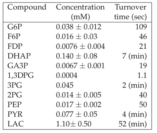
A typical glycolytic flux in the red cell is about 1.25 mM/hr. By using this number and measured concentrations, we can estimate the turnover times for the intermediates of glycolysis by simply using:
The results are shown in Table 7.5. We see the sharp distribution of turnover times that appears. Note that the turnover times are set by the relative concentrations since the flux through the pathway is the same. Thus the least abundant metabolites will have the fastest turnover. At a constant flux, the relative concentrations are set by the kinetic constants.
Table 7.5: Turnover times for the glycolytic intermediates in the red blood cell. The glycolytic flux is assumed to be 1.25 mM/hr = 0.35 \(\mu M/sec\) and the Rapoport-Luebering shunt flux is about 0.5 mM/hr. Table adapted from (Joshi, 1990).
7.2.3.3. Response of the energy charge
Exchange of high energy bonds between the various carriers is on the order of minutes. The dynamics of this energy pool occur on the middle time scale of minutes as described earlier, see Figure 7.4.
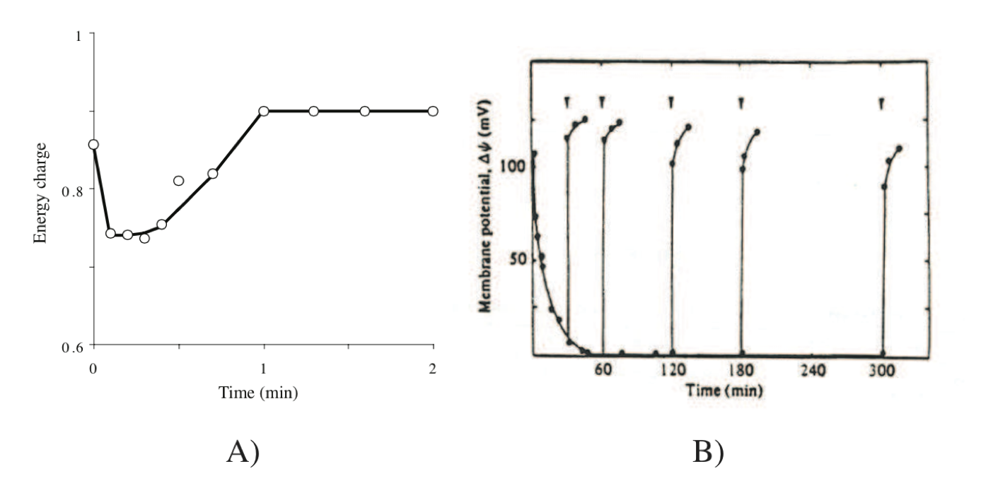
Figure 7.4: Responses in energy transduction processes in cells. (a) Effect of addition of glucose on the energy charge of Ehrlich ascites tumor cells. Redrawn based on (Atkinson, 1977). (b) Transient response of the transmembrane gradient, from (Konings, 1983). Generation of a proton motive force in energy starved S. cremoris upon addition of lactose (indicated by arrows) at different times after the start of starvation (t=0).
7.2.3.4. Response of transmembrane charge gradients
Cells store energy by extruding protons across membranes. The consequence is the formation of an osmotic and charge gradient that results in the so-called proton motive force, denoted as \(\Delta \mu_{H^+}\). It is defined by:
where \(\Delta \Psi\) is the charge gradient and \(\Delta pH\) is the hydrogen ion gradient. The parameter \(Z\) takes a value of about 60 mV under physiological conditions. The transient response of gradient establishment is very rapid, Figure 7.4.
(Konings, 1983)
7.2.3.5. Conversion between different forms of energy
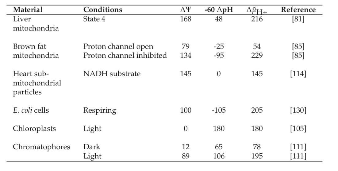
If energy is to be readily exchanged between transmembrane gradients and the high energy phosphate bond system, their displacement from equilibrium should be about the same. Based on typical ATP, ADP, and \(P_i\) concentrations, one can calculate the transmembrane gradient to be about -180mV. Table 7.6 shows that observed values for the transmembrane gradient, \(\Delta \widetilde{\mu}\), are on the order of -180 to -220 mV. It is interesting to note that the maximum gradient that a bi-lipid layer can withstand is on the order of -280mV (Konings, 1983), based on electrostatic considerations.
Table 7.6: Typical values (mV) for the transmembrane electrochemical potential gradient, reproduced from (Konings, 1983).
7.2.3.6. What are typical power densities?
The metabolic rates estimated above come with energy transmission through key cofactors. The highest energy production and dissipation rates are associated with energy transducing membranes. The ATP molecule is considered to be an energy currency of the cell, allowing one to estimate the power density in the cell/organelle based on the ATP production rate.
7.2.3.7. Power density in mitochondria
The rate of ATP production in mitochondria can be measured. Since we know the energy in each phosphate bond and the volume of the mitochondria, we can estimate the volumetric rate of energy production in the mitochondria.
Reported rates of ATP production in rat mitochondria from succinate are on the order of \(6*10^{-19}\) mol ATP/mitochondria/sec Schwerzmann86, taking place in a volume of about 0.27 \(\mu m^3\). The energy in the phosphate bond about is -52kJ/mol ATP at physiological conditions. These numbers lead to the computation of a per unit volume energy production rate of \(2.2*10^{-18}\) mol ATP/\(\mu m^3/sec\), or \(10^{-13}W/\mu m^3\ (0.1 pW/\mu m^3)\).
7.2.3.8. Power density in chloroplast of green algae
In Chlamydomonas reinhardtii, the rate of ATP production of chloroplast varies between \(9.0*10^{-17}\ \text{to}\ 1.4*10^{-16}\) mol ATP/chloroplast/sec depending on the light intensity (Baroli 2003, Burns 1990, Melis 2000, Ross 1995) in the volume of 17.4 \(\mu m^3\) (Harris 1989a). Thus, the volumetric energy production rate of chloroplast is on the order of \(5*10^{-18}\) mol ATP/\(\mu m^3/sec\), or \(3*10^{-13}W/\mu m^3\ (0.3 pW/\mu m^3)\).
7.2.3.9. Power density in rapidly growing E. coli cells:
A similar estimate of energy production rates can be performed for microorganisms. The aerobic glucose consumption of E. coli is about 10 mmol/gDW/hr. The weight of a cell is about \(2.8*10^{-13}\) gDW/cell. The ATP yield on glucose is about 17.5 ATP/glucose. These numbers allow us to compute the energy generation density from the ATP production rate of \(1.4*10^{-17}\) mol ATP/cell/sec. These numbers lead to the computation of the power density of or \(7.3*10^{-13}W/\mu m^3 O_2\ (0.7 pW/\mu m^3)\)., that is a similar numbers computed for the mitochondria and chloroplast above.
7.3. Macromolecules
We now look at the abundance, concentration and turnover rates of macromolecules in the bacterial cell. We are interested in the genome, RNA and protein molecules.
7.3.1. What are typical characteristics of a genome?
Sizes of genomes vary significantly amongst different organisms, see Table 7.7. For bacteria, they vary from about 0.5 to 9 million base pairs. The key features of the E. coli K-12 MG1655 genome are summarized in Table 7.8. There are about 4500 ORFs on the genome of an average length of about 1kb. This means that the average protein size is 316 amino acids, see Figure 7.3c.
Table 7.7: Genome sizes. A selection of representative genome sizes from the rapidly growing list of organisms whose genomes have been sequenced. Adapted from Kimball’s Biology Pages.
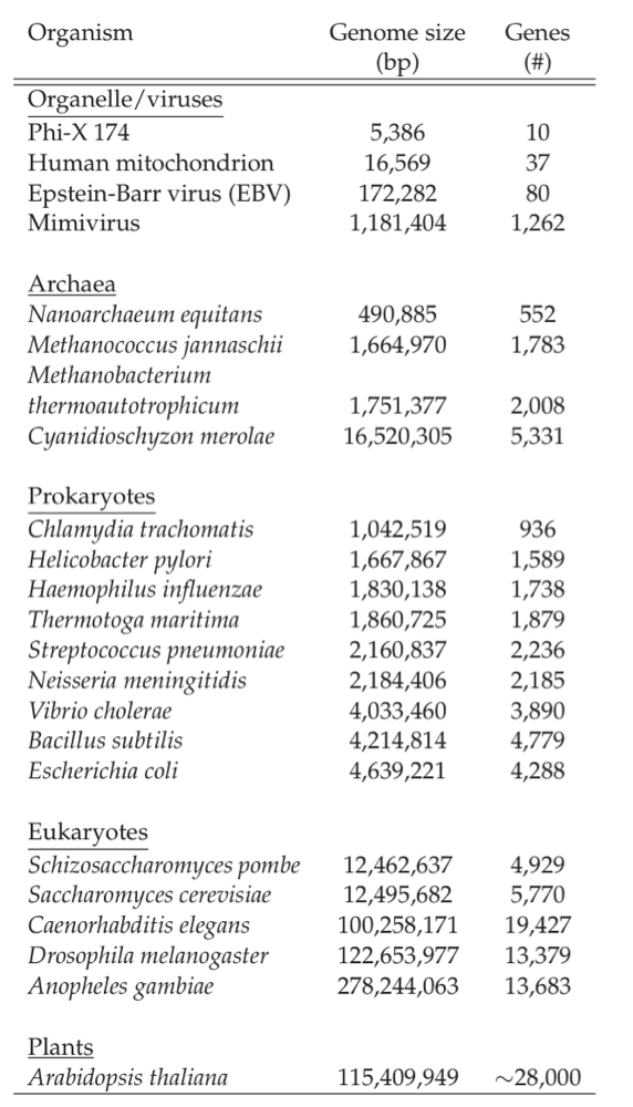
Table 7.8: Some features of the E. coli genome. From (Blattner 1997).
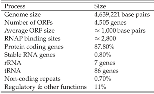
The number of RNA polymerase binding sites is estimated to be about 2800, leading to a estimate of about 1.6 ORFs \((\approx 4.4*10^6/2400)\) per transcription unit. There are roughly 3000 copies of the RNA polymerase present in an E. coli cell (Wagner 2000). Thus if 1000 of the transcription units are active at any given time, there are only 2-3 RNA polymerase molecules available for each transcription unit. The promoters have different binding strength and thus recruit a different number of RNA polymerase molecules each. ChIP-chip data can be used to estimate this distribution.
7.3.2. What are typical protein concentrations?
Cells represent a fairly dense solution of protein. One can estimate the concentration ranges for individual enzymes in cells. If we assume that the cell has about 1000 proteins with an average molecular weight of 34.7kD, as is typical for an E. coli cell, see Figure 7.3c, and given the fact that the cellular biomass is about 15% protein, we get:
This estimate is, indeed, the range into which the in vivo concentration of most proteins fall. It corresponds to about 2500 molecules of a particular protein molecule per cubic micron. As with metabolites there is a significant distribution around the estimate of Eq. (7.15). Important proteins such as the enzymes catalyzing major catabolic reactions tend to be present in higher concentrations, and pathways with smaller fluxes have their enzymes in lower concentrations. It should be noted that we are not assuming that all these proteins are in solution; the above number should be viewed more as a molar density.
The distribution about this mean is significant, Figure 7.3d. Many of the proteins in E. coli are in concentrations as low as a few dozen per cell. The E. coli cell is believed to have about 200 major proteins which brings our estimate for the abundant ones to about 12,000 copies per cell. The E. coli cell has a capacity to carry about 2.0-2.3 million protein molecules.
7.3.3. What are typical fluxes?
The rates of synthesis of the major classes of macromolecules in E. coli are summarized in Table 7.9. The genome can be replicated in 40 min with two replication forks. This means that the speed of DNA polymerase is estimated to be
RNA polymerase is much slower at 40-50 bp/sec and the ribosomes operate at about 12-21 peptide bonds per ribosome per second.
7.3.3.1. Protein synthesis capacity in E. coli
We can estimate the number of peptide bonds (pb) produced by E. coli per second. To do so we will need the rate of peptide bond formation by the ribosome (12 to 21 bp/ribosome/sec (Bremer 1996, Dennis 1974, Young 1976)); and number of ribosomes present in the E. coli cell \((7*10^3\ \text{to} \ 7*10^4\) ribosomes/cell depending on the growth rate (Bremer 1996)). So the total number of the peptide bonds that E. coli can make per second is on the order of: \(8*10^4\ \text{to}\ 1.5*10^6\) pb/cell/sec
The average size of a protein in E. coli is about 320 amino acids. At about 45 to 60 min doubling time, the total amount of protein produced by E. coli per second is ~300 to 900 protein molecules/cell/sec. This is equivalent to \(1\ \text{to}\ 3*10^6\) molecules/cell/h as a function of growth rate, about the total number of protein per cell given above.
7.3.3.2. Maximum protein production rate from a single gene in murine cells
The total amount of the protein formed from a single gene in the mammalian cell can be estimated based on the total amount of mRNA present in the cytoplasm from a single gene, the rate of translation of the mRNA molecule by ribosomes, and the ribosomal spacing (Savinell 1989). Additional factors needed include gene dosage (here taken as 1), rate of mRNA degradation, velocity of the RNA polymerase II molecule, and the growth rate (Savinell 1989).
Murine hybridoma cell lines are commonly used for antibody production. For this cell type, the total amount of mRNA from a single antibody encoding gene in the cytoplasm is on the order of 40,000 mRNA molecules/cell (Gilmore 1979, Schibler 1978) the ribosomal synthesis rate is on the order of 20 nucleotides/sec [Potter72], and the ribosomal spacing on the mRNA is between 90-100 nucleotides (Christensen 1987, Potter 1972). Multiplying these numbers, we can estimate the protein production rate in a hybridoma cell line to be approximately 3000 - 6000 protein molecules/cell/sec.
7.3.4. What are the typical turnover times?
The assembly of new macromolecules such as RNA and proteins requires the source of nucleotides and amino acids. These building blocks are generated by the degradation of existing RNA molecules and proteins. Many cellular components are constantly degraded and synthesized. This process is commonly characterized by the turnover rates and half-lives. Intracellular protein turnover is experimentally assessed by an addition of an isotope-labeled amino acid mixture to the normally growing or non-growing cells (Levine 1965, Pratt 2002). It has been shown that the rate of breakdown of an individual proteins is on the order of 2-20% per hour in E. coli culture (Levine 1965, Neidhardt 1996).
7.4. Cell Growth and Phenotypic Functions
7.4.1. What are typical cell-specific production rates?
The estimated rates of metabolism and macromolecular synthesis can be used to compute various cellular functions and their limitations. Such computations can in turn be used for bioengineering design purposes, environmental roles and impacts of microorganisms, and for other purposes. We provide a couple of simple examples.
7.4.1.1. Limits on volumetric productivity
E. coli is one of the most commonly used host organisms for metabolic engineering and overproduction of metabolites. In many cases, the glycolytic flux acts as a carbon entry point to the pathway for metabolite overproduction (Eiteman 2008, Jantama 2008, Yomano 2008, Zhu 2008). Thus, the substrate uptake rate (SUR) is one of the critical characteristics of the productive capabilities of the engineered cell.
Let us examine the wild-type E. coli grown on glucose under anoxic conditions. As shown in Table 7.4, the (SUR) is on the order of 15-20 mmol glucose/gDW/h which translates into 1.5 gm glucose/L/h at cell densities of (VP has number). Theoretically, if all the carbon source (glucose) is converted to the desired metabolite the volumetric productivity will be approximately 3 g/L/h.
The amount of cells present in the culture, play a significant role in production potential. In the industrial settings, the cell density is usually higher which increases the volumetric productivity. Some metabolic engineered strain designs demonstrate higher SUR (Portnoy 2008) that also leads to the increase in volumetric productivity.
7.4.1.2. Photoautotrophic growth
Chlorella vulgaris is a single-celled green algae that uses light to generate energy necessary for growth. At the top rate of photosynthesis, the specific oxygen production rate (SOPR) can be estimated to be between 20-400 fmol \(O_2\)/cell/h (Lee 1994a). Algae biotechnology is drawing increasing interest due to its potential for production of biofuels and fine chemicals (Lee 1994a). However, a lack of suitable photobioreactors (PBR) makes the cost of algally-derived compounds high. One of the key limiting factors for PBR is the light source; however, light-emitting diodes (LED) can be employed for these purposes.
Let us now use order of magnitude calculations to estimate the light requirement for an algae photobioreactor using C. vulgaris as a model organism. Given the fact that maximum photosynthetic efficiency of C. vulgaris is below 50% (Kok 1960, Myers 1980, Pirt 1980) and one mole of photons (680 nm) is equivalent to 50W, we can estimate that in order to sustain the SOPR of 100 fmol \(\text{O}_2\)/cell/h each cell must receive 40pW equivalent of photons (Lee1994a). A conventional LED can provide \(0.3\ \text{mW/cm}^2\) or \(0.1\ \text{mW}\) per LED. With a cell density close to \(10^9\ \text{cells/ml}\) and \(80\ \text{cm}^3\) volume of the reactor (Lee 1994a), the photobioreactor must include close to a 100 LED to sustain the growth of algae and oxygen production.
7.4.2. Balancing the fluxes and composition in an entire cell
The approximate calculation procedures presented can be used to estimate the overall flows of mass and energy in a bacterial cell. Proteins are 55% of the dry weight of cells and their most energetically costly component, so let’s begin such computation with the assumption that there are about \(10^9\) amino acids found in the proteins of a single cell. With this starting point and the various data given in this chapter, we can roughly estimate all the major flows using a 60 min doubling time:
With approximately 316 amino acids found in a protein, we have to make about 3 million protein molecules.
If we take the ribosome to make 20 pb/sec = 72,000 pb/hr, (pb=peptide bond) the we require
\[\begin{equation} \frac{1,000,000,000}{72,000} = 14,000\ \text{ribosomes} \tag{7.17} \end{equation}\]to carry out this protein synthesis.
To make 14,000 ribosomes with each having 4,500 nt length RNA molecules (nt = nucleotide), we need
\[\begin{equation} 14,000*4,500 = 63,000,000\ \text{nt}\ \tag{7.18} \end{equation}\]assembled. In addition, there are 10 tRNAs of 80 nt in length per ribosome leading to an additional nucleotide requirement of
\[\begin{equation} 10*80*14,000 = 11,200,000\ \text{nt}\ \tag{7.19} \end{equation}\]for a grand total of approximately 75,000,000 for stable RNA molecule synthesis.
The total nucleotide synthesis for RNA will be 3000 RNA polymerase molecules synthesizing at the rate of 50 nt/sec or
\[\begin{equation} 3000*50*3600 = 540,000,000\ \text{nt/hour}\ \tag{7.20} \end{equation}\]The fraction of RNA that is mRNA is 0.03 to 0.05 Rosenow01 or,
\[\begin{equation} 540,000,000*(0.03\ \text{to}\ 0.05) \approx (16\ \text{to}\ 25.0)*10^6\ \text{nt/cell/hr}\ \tag{7.21} \end{equation}\]If the average mRNA length is 1100 nt then the cell needs to make on average 20,000 transcripts in one hour.
We have to make 3,000,000 proteins from 20,000 transcripts, or about 150 protein molecules per transcript.
The transcripts have a finite half live. On average, each transcript has a 5 min lifetime, or 300 sec. Due to structural constraints a ribosome can only bind every 50 nt to the mRNA, producing a maximum ribosomal loading of about 20 ribosomes per transcript. The rate of translation is 20 pb/sec. With the average length of the peptide being 316 amino acids, we can produce 1.25 protein/sec. This calculation estimated the maximum protein production from one transcript on the order of 375 protein molecules per transcript.
To synthesize the genome, we need \(2*4,500,000 = 9,000,000\ \text{nt}\) to make the double stranded DNA.
Thus, the total metabolic requirement of amino acids and nucleotides in E. coli per doubling is \(1*10^9\) amino acids/cell/h and \(5*10^8\) nt/cell/h.
These are the approximate overall material requirements. We also need energy to drive the process. Using Table 7.4 we can estimate energy requirements for E. coli under oxic and anoxic conditions.
Aerobically, at a doubling time of 1 hour, the glucose uptake rate is about 10 mmol/gDW/h, that is equivalent to \(1.5*10^9\) molecules of glucose per cell per doubling. At 17.5 ATP produced per glucose he corresponding energy production is: \(3*10^{10}\) ATP per cell per doubling.
Anaerobically, at a doubling time of 1.5 hours, the glucose uptake rate is about 18 mmol/gDW/h, which is equivalent to \(4.5*10^9\) molecules of glucose/ cell/doubling. At 3 ATP per glucose the corresponding energy production is \(1.4*10^{10}\) molecules ATP/cell/doubling.
7.5. Summary
Data on cellular composition and over all rates are available.
Order of magnitude estimation procedures exist through which one can obtain the approximate values for key quantities.
In this fashion, typical concentrations, fluxes and turnover times can be estimated.
An approximate quantitative overall multi-scale framework can be obtained for the function of complex biological processes.
\(\tiny{\text{© B. Ø. Palsson 2011;}\ \text{This publication is in copyright.}\\ \text{Subject to statutory exception and to the provisions of relevant collective licensing agreements,}\\ \text{no reproduction of any part may take place without the written permission of Cambridge University Press.}}\)