1. Introduction

Systems biology has been brought to the forefront of life science-based research and development. The need for systems analysis is made apparent by the inability of focused studies to explain whole network, cell, or organism behavior, and the availability of component data is what is fueling and enabling the effort. This massive amount of experimental information is a reflection of the complex molecular networks that underlie cellular functions. Reconstructed networks represent a common denominator in systems biology. They are used for data interpretation, comparing organism capabilities, and as the basis for computing their functional states. The companion book Systems Biology: Properties of Reconstructed Networks details the topological features and assessment of functional states of biochemical reaction networks and how these features are represented by the stoichiometric matrix. In this book, we turn our attention to the kinetic properties of the reactions that make up a network. We will focus on the formulation of dynamic simulators and how they are used to generate and study the dynamic states of biological networks.

1.1. Biological Networks

Cells are made up of many chemical constituents that interact to form networks. Networks are fundamentally comprised of nodes (the compounds) and the links (chemical transformations) between them. The networks take on functional states that we wish to compute, and it is these physiological states that we observe. This text is focused on dynamic states of networks.

There are many different kinds of biological networks of interest, and they can be defined in different ways. One common way to define networks is based on a preconceived notion of what they do. Examples include metabolic, signaling, and regulatory networks, see Figure 1.1. This approach is driven by a large body of literature that has grown around a particular cellular function.

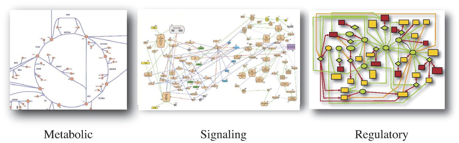
Figure 1.1: Three examples of networks that are defined by major function. (a) Metabolism. (b) Signaling. From Arisi, et al. BMC Neuroscience 2006 7(Suppl 1):S6 DOI:10.1186/1471-2202-7-S1-S6. (c) Transcriptional regulatory networks. Image courtesy of Christopher Workman, Center for Biological Sequence Analysis, Technical University of Denmark.

1.1.1. Metabolic networks

Metabolism is ubiquitous in living cells and is involved in essentially all cellular functions. It has a long history - glycolysis was the first pathway elucidated in the 1930s - and is thus well-known in biochemical terms. Many of the enzymes and the corresponding genes have been discovered and characterized. Consequently, the development of dynamic models for metabolism is the most advanced at the present time.

A few large-scale kinetic models of metabolic pathways and networks now exist. Genome-scale reconstructions of metabolic networks in many organisms are now available. With the current developments in metabolomics and fluxomics, there is a growing number of large-scale data sets becoming available. However, there are no genome-scale dynamic models yet available for metabolism.

1.1.2. Signaling networks

Living cells have a large number of sensing mechanisms to measure and evaluate their environment. Bacteria have a surprising number of 2-component sensing systems that inform the organism about its nutritional, physical, and biological environment. Human cells in tissues have a large number of receptor systems in their membranes to which specific ligands bind, such as growth factors or chemokines. Such signaling influences the cellular fate processes: differentiation, replication, apoptosis, and migration.

The function of many of the signaling pathways that is initiated by a sensing event are presently known, and this knowledge is becoming more detailed. Only a handful of signaling networks are well-known, such as the JAK-STAT signaling network in lymphocytes and the Toll-like receptor system in macrophages. A growing number of dynamic models for individual signaling pathways are becoming available.

1.1.3. Regulatory networks

There is a complex network of interactions that determine the DNA binding state of most proteins, which in turn determine if genes are being expressed. The RNA polymerase must bind to DNA, as do transcription factors and various other proteins. The details of these chemical interactions are being worked out, but in the absence of such information, most of the network models that have been built are discrete, stochastic, and logistical in nature.

With the rapid development of experimental methods that measure expression states, the binding sites, and their occupancy, we may soon see large-scale reconstructions of transcriptional regulatory networks. Once these are available, we can begin to plan the process to build models that will describe their dynamic states.

1.1.4. Unbiased network definitions

An alternative way to define networks is based on chemical assays. Measuring all protein-protein interactions regardless of function provides one such example, see Figure 1.2. Another example is a genome-wide measurement of the binding sites of a DNA-binding protein. This approach is driven by data-generating capabilities. It does not have an a priori bias about the function of molecules being examined.

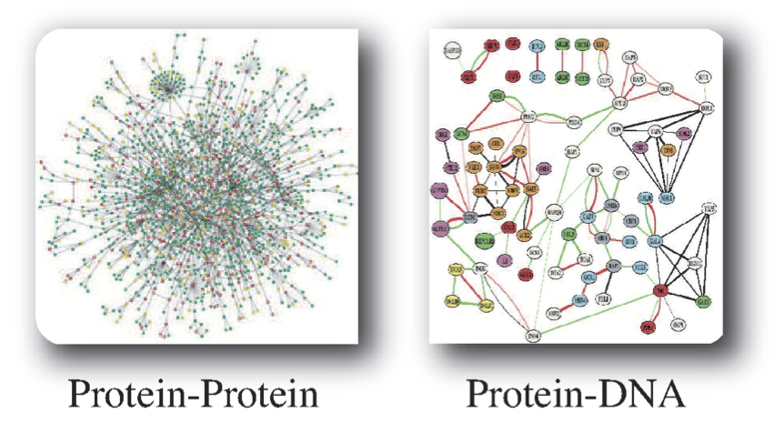
Figure 1.2: Two examples of networks that are defined by high-throughput chemical assays. Images courtesy of Markus Herrgard.

1.1.5. Network reconstruction

Metabolic networks are currently the best-characterized biological networks for which the most detailed reconstructions are available. The conceptual basis for their reconstruction has been reviewed (Reed, 2006), the workflows used detailed (Feist, 2009) and a detailed standard operating procedure (SOP) is available (Thiele, 2010). Some of the fundamental issues associated with the generation of dynamic models describing their functions have been articulated (Jashmidi, 2008).

There is much interest in reconstructing signaling and regulatory networks in a similar way. The prospects for reconstruction of large-scale signaling networks have been discussed (Hyduke, 2010). Given the development of new omics data types and other information, it seems likely that we will be able to obtain reliable reconstructions of these networks in the not too distant future.

1.1.6. Public information about pathways and networks

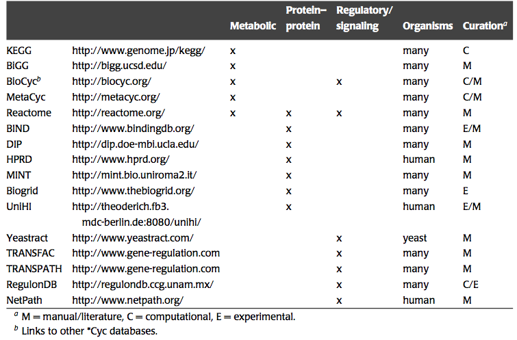
There is a growing number of networks that underlie cellular functions that are being unraveled and reconstructed. Many publicly available sources contain this information, Table 1.1. We wish to study the dynamic states of such networks. To do so, we need to describe them in chemical detail and incorporate thermodynamic information and formulate a mathematical model.

Table 1.1: Web resources that contain information about biological networks. Prepared by Jan Schellenberger.

1.2. Why Build and Study Models?

Mathematical modeling is practiced in various branches of science and engineering. The construction of models is a laborious and detailed task. It also involves the use of numerical and mathematical analysis, both of which are intellectually intensive and unforgiving undertakings. So why bother?

1.2.1. Bailey’s five reasons

The purpose and utility of model building has been succinctly summarized and discussed (Bailey, 1998):

1. “To organize disparate information into a coherent whole.” The information that goes into building models is often found in many different sources and the model-builder has to look for these, evaluate them, and put them in context. In our case, this comes down to building data matrices (see Table 1.3) and determining conditions of interest.

2. “To think (and calculate) logically about what components and interactions are important in a complex system.” Once the information has been gathered it can be mathematically represented in a self-consistent format. Once equations have been formulated using the information gathered and according to the laws of nature, the information can be mathematically interrogated. The interactions among the different components are evaluated and the behavior of the model is compared to experimental data.

3. “To discover new strategies.” Once a model has been assembled and studied, it often reveals relationships among its different components that were not previously known. Such observations often lead to new experiments, or form the basis for new designs. Further, when a model fails to reproduce the functions of the process being described, it means there is either something critical missing in the model or the data that led to its formulation is inconsistent. Such an occurrence then leads to a re-examination of the information that led to the model formulation. If no logical flaw is found, the analysis of the discrepancy may lead to new experiments to try to discover the missing information.

4. “To make important corrections to the conventional wisdom.” The properties of a model may differ from the governing thinking about process phenomena that is inferred based on qualitative reasoning. Good models may thus lead to important new conceptual developments.

5. “To understand the essential qualitative features.” Since a model accounts for all described interactions among its parts, it often leads to a better understanding of the whole. In the present case, such qualitative features relate to multi-scale analysis in time and an understanding of how multiple chemical events culminate in coherent physiological features.

1.3. Characterizing Dynamic States

The dynamic analysis of complex reaction networks involves the tracing of time-dependent changes of concentrations and reaction fluxes over time. The concentrations typically considered are those of metabolites, proteins, or other cellular constituents. There are three key characteristics of dynamics states that we mention here right at the outset, and they are described in more detail in Section 2.1.

1.3.1. Time constants

Dynamic states are characterized by change in time, thus the rate of change becomes the key consideration. The rate of change of a variable is characterized by a time constant. Typically, there is a broad spectrum of time constants found in biochemical reaction networks. This leads to time scale separation where events may be happening on the order of milliseconds all the way to hours, if not days. The determination of the spectrum of time constants is thus central to the analysis of network dynamics.

1.3.2. Aggregate variables

An associated issue is the identification of the biochemical, and ultimately physiological, events that are unfolding on every time scale. Once identified, one begins to form aggregate concentration variables, or pooled variables. These variables will be combinations of the original concentration variables. For example, two concentration variables may inter-convert rapidly, on the order of milliseconds, and thus on every time scale longer than milliseconds, these two concentrations will be “connected.” They can therefore be “pooled” together to form an aggregate variable. An example is given in Figure 1.3.

The determination of such aggregate variables becomes an intricate mathematical problem. Once solved, it allows us to determine the dynamic structure of a network. In other words, we move hierarchically away from the original concentration variables to increasingly interlinked aggregate variables that ultimately culminate in the overall dynamic features of a network on slower time scales. Temporal decomposition therefore involves finding the time scale spectrum of a network and determining what moves on each one of these time scales. A network can then be studied on any one of these time scales.

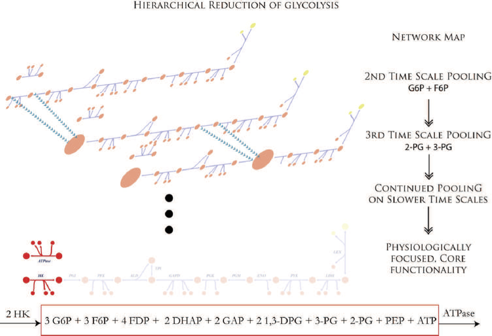
Figure 1.3: Time-scale hierarchy and the formation of aggregate variables in glycolysis.The ‘pooling’ process culminates in the formation of one pool (shown in a box at the bottom) that is filled by hexokinase (HK) and drained by ATPase. This pool represents the inventory of high energy phosphate bonds. From (Jashmidi, 2008).

1.3.3. Transitions

Complex networks can transition from one steady state (i.e., homeostatic state) to another. There are distinct types of transitions that characterize the dynamic states of a network. Transitions are analyzed by bifurcation theory. The most common bifurcations involve the emergence of multiple steady states, sustained oscillations, and chaotic behavior. Such dynamic features call for a yet more sophisticated mathematical treatment. Such changes in dynamic states have been called creative functions, which in turn represent willful physiological changes in organism behavior. In this book, we will only encounter relatively simple types of such transitions.

1.4. 1.4 Formulating Dynamic Network Models

1.4.1. Approach

Mechanistic kinetic models based on differential equations represent a bottom-up approach. This means that we identify all the detailed events in a network and systematically build it up in complexity by adding more and more new information about the components of a network and how they interact. A complementary approach to the analysis of a biochemical reaction network is a top-down approach where one collects data and information about the state of the whole network at one time. This approach is not covered in this text but typically requires a Bayesian or Boolean analysis that represents causal or statistically-determined relationships between network components. The bottom-up approach requires a mechanistic understanding of component interactions. Both the top-down and bottom-up approaches are useful and complimentary in studying the dynamic states of networks.

1.4.2. Simplifying assumptions

Kinetic models are typically formulated as a set of deterministic ordinary differential equations (ODEs). There are a number of important assumptions made in such formulations that often are not fully described and delineated. Five assumptions will be discussed here (Table 1.2).

Table 1.2: Assumptions used in the formulation of biological network models.

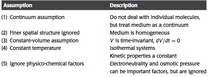
1. Using deterministic equations to model biochemistry essentially implies a “clockwork” of functionality. However, this modeling assumption needs justification. There are three principal sources of variability in biological dynamics: internal thermal noise, changes in the environment, and cell-to-cell variation. Inside cells, all components experience thermal effects that result in random molecular motion. This process is, of course, one of molecular diffusion, called Brownian motion with larger observable objects. The ordinary differential equation assumption involves taking an ensemble of molecules and averaging out the stochastic effects. In cases where there are very few molecules of a particular species inside a cell or a cellular compartment, this assumption may turn out to be erroneous.

2. The finer architecture of cells is also typically not considered in kinetic models. Cells are highly structured down to the 100 nm length scale and are thus not homogeneous (see Figure 1.4). Rapidly diffusing compounds, such as metabolites and ions, will distribute rapidly throughout the compartment and one can justifiably consider the concentration to be relatively uniform. However, with larger molecules whose diffusion is hindered and confined, one may have to consider their spatial location. Studying and describing cellular functions of the 100 nm length scale is likely to represent an interesting topic in systems biology as it unfolds.

3. Another major assumption in most kinetic models is that of constant volume. Cells and cellular compartments typically have fluctuations in their volume. Treating variable volume turns out to be mathematically difficult. It is, therefore, often ignored. However, minor fluctuations in the volume of a cellular compartment may change all the concentrations in that compartment and therefore all kinetic and regulatory effects.

4. Temperature is typically considered to be a constant. Larger organisms have the capability to control their temperature. Small organisms have a high surface to volume ratio making it hard to control heat flux at their periphery. Further, small cellular dimensions lead to rapid thermal diffusivity and a strong dependency on the thermal characteristics of the environment. Rate constants are normally a strong function of temperature, often described by Arrhenius’ law. Thus, treating cells as isothermal systems is a simplification under which the kinetic properties are described by kinetic constants.

5. All cells and cellular compartments must maintain electro-neutrality and therefore the exchange of any species in and out of a compartment or a cell must also obey electro-neutrality. Considering the charge of molecules and their pH dependence is yet another complicated mathematical subject and thus often ignored. Similarly, significant internal osmotic pressure must be balanced with that of the environment. Cells in tissues are in an isotonic environment, while single cellular organisms and cells in plants build rigid walls to maintain their integrity.

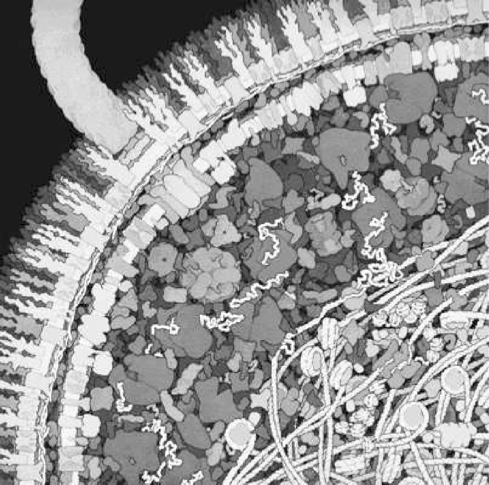
Figure 1.4: The crowded state of the intracellular environment.Some of the physical characteristics are viscosity \((>100\ \mu_{H2O})\), osmotic pressure \((<150 atm)\), electrical gradients \((\approx 300,000\ V/cm)\), and a near crystalline state. © David S.Goodsell 1999.

1.4.3. The dynamic mass balance equations

Applying these simplifying assumptions, we arrive at the dynamic mass balance equations as the starting point for modeling the dynamic states of biochemical reaction networks. The basic notion of a dynamic mass balance on a single compound, \(x_i\), is shown in Figure 1.5.

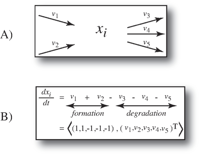
Figure 1.5: The dynamic mass balance on a single compound. (a) All the rates of formation and degradation of a compound \(x_i\) (a graphical representation called a node map). (b) The corresponding dynamic mass balance equation that simply states that the rate of change of the concentrations \(x_i\) is equal to the sum of the rates of formation minus the sum of the rates of degradation. This summation can be represented as an inner product between a row vector and the flux vector. This row vector becomes a row in the stoichiometric matrix in Eq. 1.1.

The combination of all the dynamic mass balances for all concentrations (\(\textbf{x}\))in a biochemical reaction network are given by a matrix equation:

\[\begin{equation} \frac{d\textbf{x}}{dt} = \textbf{Sv}(\textbf{x}) \tag{1.1} \end{equation}\]

where \(\textbf{S}\) is the stoichiometric matrix, \(\textbf{v}\) is the vector of reaction fluxes \((v_j)\), and \(\textbf{x}\) is the vector of concentrations \((x_i)\). Equation 1.1 will be the ‘master’ equation that will be used to describe network dynamics states in this book.

1.4.4. Alternative views

There are a number of considerations that come with the differential equation formalism described in this book and in the vast majority of the research literature on this subject matter. Perhaps the most important issue is the treatment of cells as behaving deterministically and displaying continuous changes over time. It is possible, though, that cells ultimately will be viewed as essentially a liquid crystalline state where transitions will be discreet from one state to the next, and not continuous.

1.5. The Basic Information is in a Matrix Format

The natural mathematical language for describing network states using dynamic mass balances is that of matrix algebra. In studying the dynamic states of networks, there are three fundamental matrices of interest: the stoichiometric, the gradient, and the Jacobian matrices.

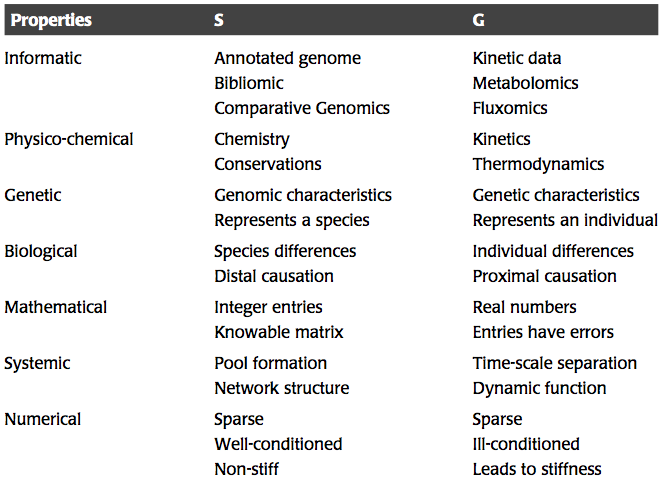
Table 1.3: Comparison of some of the attributes and properties of the stoichiometric and the gradient matrices. Adapted from (Jashmidi, 2008).

1.5.1. The stoichiometric matrix

The stoichiometric matrix, the properties of which are detailed in (SB1), represents the reaction topology of a network. Every row in this matrix represents a compound (alternative states require multiple rows) and every column represents a link between compounds, or a chemical reaction. All the entries in this matrix are stoichiometric coefficients. This matrix is “knowable,” since it is comprised of integers that have no error associated with them. The stoichiometric matrix is genomically-derived and thus all members of a species or a biopopulation will have the same stoichiometric matrix.

Mathematically, the stoichiometric matrix has important features. It is a sparse matrix, which means that few of its elements are non-zero. Typically, less than 1% of the elements of a genome-scale stoichiometric matrix are non-zero, and those non-zero elements are almost always 1 or -1. Occasionally there will be an entry of numerical value 2, which may represent the formation of a homodimer. The fact that all the elements of \(\textbf{S}\) are of the same order of magnitude makes it a convenient matrix to deal with from a numerical standpoint. The properties of the stoichiometric matrix have been extensively studied (SB1).

1.5.2. The gradient matrix

Each link in a reaction map has kinetic properties with which it is associated. The reaction rates that describe the kinetic properties are found in the rate laws, \(\textbf{v}(\textbf{x}; \textbf{k})\), where the vector \(\textbf{k}\) contains all the kinetic constants that appear in the rate laws. Ultimately, these properties represent time constants that tell us how quickly a link in a network will respond to the concentrations that are involved in that link. The reciprocal of these time constants are found in the gradient matrix, \(\textbf{G}\), whose elements are:

\[\begin{equation} g_{ij} = \frac{\partial v_i}{\partial x_j}[\text{time}^{-1}] \tag{1.2} \end{equation}\]

These constants may change from one member to the next in a biopopulation given the natural sequence diversity that exists. Therefore, the gradient matrix, is a genetically-determined matrix. Two members of the population may have a different \(\textbf{G}\) matrix. This difference is especially important in cases where mutations exist that significantly change the kinetic properties of critical steps in the network and change its dynamic structure. Such changes in the properties of a single link in a network may change the properties of the entire network.

Mathematically speaking, \(\textbf{G}\) has several challenging features. Unlike the stoichiometric matrix, its numerical values vary over many orders of magnitude. Some links have very fast response times, while others have long response times. The entries of \(\textbf{G}\) are real numbers and therefore are not “knowable.” The values of \(\textbf{G}\) will always come with an error bar associated with the experimental method used to determine them. Sometimes only order-of-magnitude information about the numerical values of the entries in \(\textbf{G}\) is sufficient to allow us to determine the overall dynamic properties of a network. The matrix \(\textbf{G}\) has the same sparsity properties as the matrix \(\textbf{S}\).

1.5.3. The Jacobian matrix

The Jacobian matrix, \(\textbf{J}\), is the matrix that characterizes network dynamics. It is a product of the stoichiometric matrix and the gradient matrix. The stoichiometric matrix gives us network structure, and the gradient matrix gives us kinetic parameters of the links in the network. The product of these two matrices gives us the network dynamics.

The three matrices described above are thus not independent. The Jacobian is given by

\[\begin{equation} \textbf{J} = \textbf{SG} \tag{1.3} \end{equation}\]

The properties of \(\textbf{S}\) and \(\textbf{G}\) are compared in Table 1.3.

1.6. Summary

• Large-scale biological networks that underlie various cellular functions can now be reconstructed from detailed data sets and published literature.

• Mathematical models can be built to study the dynamic states of networks. These dynamic states are most often described by ordinary differential equations.

• There are significant assumptions leading to an ordinary differential equations formalism to describe dynamic states. Most notably is the elimination of molecular noise, assuming volumes and temperature to be constant, and considering spatial structure to be insignificant.

• Networks have dynamic states that are characterized by time constants, pooling of variables, and characteristic transitions. The basic dynamic properties of a network come down to analyzing the spectrum of time-scales associated with a network and how the concentrations move on these time-scales.

• Sometimes the concentrations move in tandem at certain time-scales, leading to the formation of aggregate variables. This property is key to the hierarchical decomposition of networks and the understanding of how physiological functions are formed.

• The data used to formulate models to describe dynamic states of networks is found in two matrices: the stoichiometric matrix, that is typically well-known, the gradient matrix, whose elements are harder to determine.

• Dynamic states can be studied by simulation or mathematical analysis. This text is focused on the process of dynamic simulation and its uses.

\(\tiny{\text{© B. Ø. Palsson 2011;}\ \text{This publication is in copyright.}\\ \text{Subject to statutory exception and to the provisions of relevant collective licensing agreements,}\\ \text{no reproduction of any part may take place without the written permission of Cambridge University Press.}}\)