2. Basic Concepts
The bottom-up analysis of dynamic states of a network is based on network topology and kinetic theory describing the links in the network. In this chapter, we provide a primer for the basic concepts of dynamic analysis of network states. We also discuss basics of the kinetic theory that is needed to formulate and understand detailed dynamic models of biochemical reaction networks.
2.1. Properties of Dynamic States
The three key dynamic properties outlined in the introduction - time constants, aggregate variables and transitions - are detailed in this section.
2.1.1. Time scales
A fundamental quantity in dynamic analysis is the time constant. A time constant is a measure of time span over which significant changes occur in a state variable. It is thus a scaling factor for time and determines where in the time scale spectrum one needs to focus attention when dealing with a particular process or event of interest.
A general definition of a time constant is given by
where \(\Delta{x}\) is a characteristic change in the state variable \(x\) of interest and \(|dx/dt|_{avg}\) is an estimate of the rate of change of the variable \(x\). Notice the ratio between \(\Delta{x}\) and the average derivative has units of time, and the time constant characterizes the time span over which these changes in \(x\) occur, see Figure 2.1.
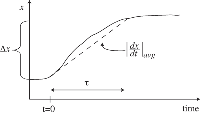
Figure 2.1: Illustration of the concept of a time constant, \(\tau\), and its estimation as \(\tau = \Delta x\ / |dx/dt|_{avg}.\)
In a network, there are many time constants. In fact, there is a spectrum of time constants, \(\tau_1,\ \tau_2, \dots \tau_r\) where \(r\) is the rank of the Jacobian matrix defining the dynamic dimensionality of the dynamic response of the network. This spectrum of time constants typically spans many orders of magnitude. The consequences of a well-separated set of time constants is a key concern in the analysis of network dynamics.
2.1.2. Forming aggregate variables through “pooling”
One important consequence of time scale hierarchy is the fact that we will have fast and slow events. If fast events are filtered out or ignored, one removes a dynamic degree of freedom from the dynamic description, thus reducing the dynamic dimension of a system. Removal of a dynamic dimension leads to “coarse-graining” of the dynamic description. Reduction in dynamic dimension results in the combination, or pooling, of variables into aggregate variables.
A simple example can be obtained from upper glycolysis. The first three reactions of this pathway are:
This schema includes the second step in glycolysis where glucose-6-phosphate (G6P) is converted to fructose-6-phosphate (F6P) by the phosphogluco-isomerase (PGI). Isomerases are highly active enzymes and have rate constants that tend to be fast. In this case, PGI has a much faster response time than the response time of the flanking kinases in this pathway, hexokinase (HK) and phosphofructokinase (PFK). If one considers a time period that is much greater than \(\tau_f\) (the time constant associated with PGI), this system is simplified to:
where HP = (G6P+F6P) is the hexosephosphate pool. At a slow time scale (i.e, long compared to \(\tau_f\)), the isomerase reaction has effectively equilibrated, leading to the removal of its dynamics from the network. As a result, F6P and G6P become dynamically coupled and can be considered to be a single variable. HP is an example of an aggregate variable that results from pooling G6P and F6P into a single variable. Such aggregation of variables is a consequence of time-scale hierarchy in networks. Determining how to aggregate variables into meaningful quantities becomes an important consideration in the dynamic analysis of network states. Further examples of pooling variables are given in Section 2.3.
2.1.3. Transitions
The dynamic analysis of a network comes down to examining its transient behavior as it moves from one state to another.
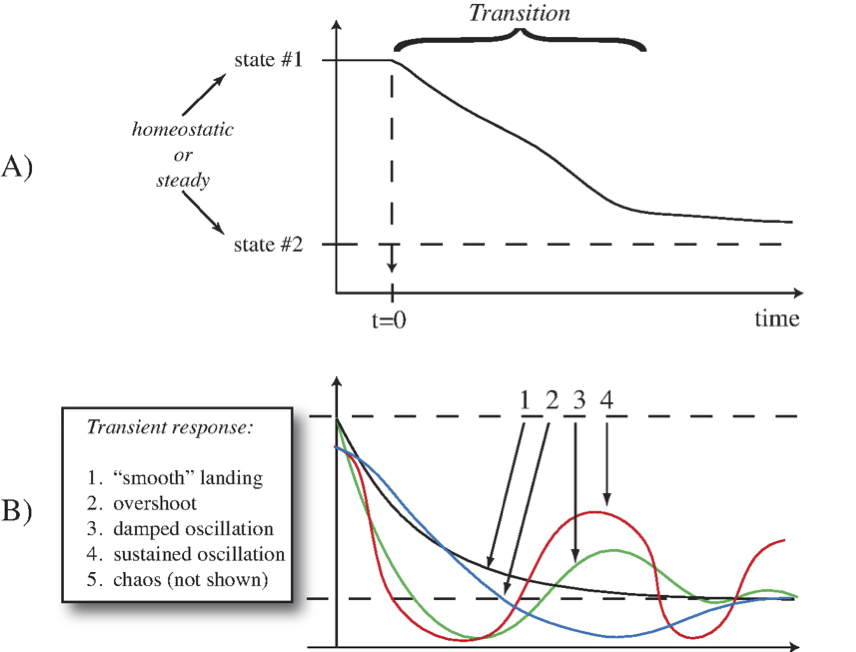
Figure 2.2: Illustration of a transition from one state to another. (a) A simple transition. (b) A more complex set of transitions.
One type of transition, or transient response, is illustrated in Figure 2.2a, where a system is in a homeostatic state, labeled as state \(\text{#1}\), and is perturbed at time zero. Over some time period, as a result of the perturbation, it transitions into another homeostatic state (state \(\text{#2}\)). We are interested in characteristics such as the time duration of this response, as well as looking at the dynamic states that the network exhibits during this transition. Complex types of transitions are shown in Figure 2.2b.
It should be noted that when complex kinetic models are studied, there are two ways to perturb a system and induce a transient response. One is to instantaneously change the initial condition of one of the state variables (typically a concentration), and the second is to change the state of an environmental variable that represents an input to the system. The latter perturbation is the one that is biologically meaningful, whereas the former may be of some mathematical interest.
2.1.4. Visualizing dynamic states
There are several ways to graphically represent dynamic states:
First, we can represent them on a map (Figure 2.3a). If we have a reaction or a compound map for a network of interest, we can simply draw it out on a computer screen and leave open spaces above the arrows and the concentrations into which we can write numerical values for these quantities. These quantities can then be displayed dynamically as the simulation proceeds, or by a graph showing the changes in the variable over time. This representation requires writing complex software to make such an interface.
A second, and probably more common, way of viewing dynamic states is to simply graph the state variables, \(x\), as a function of time (Figure 2.3b). Such graphs show how the variables move up and down, and on which time scales. Often, one uses a logarithmic scale for the y-axis, and that often delineates the different time constants on which a variable moves.
A third way to represent dynamic solutions is to plot two state variables against one another in a two-dimensional plot (Figure 2.3c). This representation is known as a phase portrait. Plotting two variables against one another traces out a curve in this plane along which time is a parameter. At the beginning of the trajectory, time is zero, and at the end, time has gone to infinity. These phase portraits will be discussed in more detail in Chapter 3.
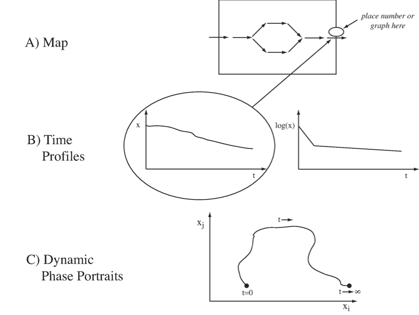
Figure 2.3: Graphical representation of dynamic states.
2.2. Primer on Rate Laws
The reaction rates, \(v_i\), are described mathematically using kinetic theory. In this section, we will discuss some of the fundamental concepts of kinetic theory that lead to their formation.
2.2.1. Elementary reactions
The fundamental events in chemical reaction networks are elementary reactions. There are two types of elemental reactions:
A special case of a bi-linear reaction is when \(x_1\) is the same as \(x_2\) in which case the reaction is second order.
Elementary reactions represent the irreducible events of chemical transformations, analogous to a base pair being the irreducible unit of DNA sequence. Note that rates, \(v\), and concentrations, \(x\), are non-negative variables, that is;
2.2.2. Mass action kinetics
The fundamental assumption underlying the mathematical description of reaction rates is that they are proportional to the collision frequency of molecules taking part in a reaction. Most commonly, reactions are bi-linear, where two different molecules collide to produce a chemical transformation. The probability of a collision is proportional to the concentration of a chemical species in a 3-dimensional unconstrained domain. This proportionality leads to the elementary reaction rates:
2.2.3. Enzymes increase the probability of the ‘right’ collision
Not all collisions of molecules have the same probability of producing a chemical reaction. Collisions at certain angles are more likely to produce a reaction than others. As illustrated in Figure 2.4, molecules bound to the surface of an enzyme can be oriented to produce collisions at certain angles, thus accelerating the reaction rate. The numerical values of the rate constants are thus genetically determined as the structure of a protein is encoded in the sequence of the DNA. Sequence variation in the underlying gene in a population leads to differences amongst the individuals that make up the population. Principles of enzyme catalysis are further discussed in Section 5.1.
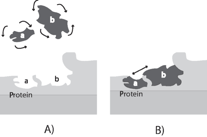
Figure 2.4: A schematic showing how the binding sites of two molecules on an enzyme bring them together to collide at an optimal angle to produce a reaction. Panel A: Two molecules can collide at random and various angles in free solution. Only a fraction of the collisions lead to a chemical reaction. Panel B: Two molecules bound to the surface of a reaction can only collide at a highly restricted angle, substantially enhancing the probability of a chemical reaction between the two compounds. Redrawn based on (Lowenstein, 2000).
2.2.4. Generalized mass action kinetics
The reaction rates may not be proportional to the concentration in certain circumstances, and we may have what are called power-law kinetics. The mathematical form of the elementary rate laws are
where \(a\) and \(b\) can be greater or smaller than unity. In cases where a restricted geometry reduces the probability of collision relative to a geometrically-unrestricted case, the numerical values of \(a\) and \(b\) are less than unity, and vice versa.
2.2.5. Combining elementary reactions
In the analysis of chemical kinetics, the elementary reactions are often combined into reaction mechanisms. Following are two such examples:
2.2.5.1. Reversible reactions:
If a chemical conversion is thermodynamically reversible, then the two opposite reactions can be combined as
The net rate of the reaction can then be described by the difference between the forward and reverse reactions;
where \(K_{eq}\) is the equilibrium constant for the reaction. Note that \(v_{net}\) can be positive or negative. Both \(k^+\) and \(k^-\) have units of reciprocal time. They are thus inverses of time constants. Similarly, a net reversible bi-linear reaction can be written as
The net rate of the reaction can then be described by
where \(K_{eq}\) is the equilibrium constant for the reaction. The units on the rate constant \((k^+)\) for a bi-linear reaction are concentration per time. Note that we can also write this equation as
that can be a convenient form as often the \(K_{eq}\) is a known number with a thermodynamic basis, and thus only a numerical value for \(k^+\) needs to be estimated.
2.2.5.2. Converting enzymatic reaction mechanisms into rate laws:
Often, more complex combinations of elementary reactions are analyzed. The classical irreversible Michaelis-Menten mechanism is comprised of three elementary reactions.
where a substrate, \(S\), binds to an enzyme to form a complex, \(X\), that can break down to generate the product, \(P\). The concentrations of the corresponding chemical species is denoted with the same lower case letter; i.e., \(e=[E]\), etc. This reaction mechanism has two conservation quantities associated with it: one on the enzyme \(e_{tot} = e + x\) and one on the substrate \(s_{tot} = s+x+p\).
A quasi-steady-state assumption (QSSA), \(dx/dt=0\), is then applied to generate the classical rate law
that describes the kinetics of this reaction mechanism. This expression is the best-known rate equation in enzyme kinetics. It has two parameters: the maximal reaction rate \(v_m\), and the Michaelis-Menten constant \(K_m = (k_{-1} + k_2)/k_1\). The use and applicability of kinetic assumptions to deriving rate laws for enzymatic reaction mechanisms is discussed in detail in Chapter 5.
It should be noted that the elimination of the elementary rates through the use of the simplifying kinetic assumptions fundamentally changes the mathematical nature of the dynamic description from that of bi-linear equations to that of hyperbolic equations (i.e., Eq. 2.9) and, more generally, to ratios of polynomial functions.
2.2.6. Pseudo-first order rate constants (PERCs)
The effects of temperature, pH, enzyme concentrations, and other factors that influence the kinetics can often be accounted for in a condition specific numerical value of a constant that looks like a regular elementary rate constant, as in Eq (2.4). The advantage of having such constants is that it simplifies the network dynamic analysis. The disadvantage is that dynamic descriptions based on PERCs are condition specific. This issue is discussed in Parts 3 and 4 of the book.
2.2.7. The mass action ratio (\(\Gamma\))
The equilibrium relationship among reactants and products of a chemical reaction are familiar to the reader. For example, the equilibrium relationship for the PGI reaction (Eq. (2.8)) is
This relationship is observed in a closed system after the reaction is allowed to proceed to equilibrium over a long time, \(t \rightarrow \infty\), (which in practice has a meaning relative to the time constant of the reaction, \(t \gg \tau_f\)).
However, in a cell, as shown in Eq. (2.2), the PGI reactions operate in an “open” environment, i.e., G6P is being produced and F6P is being consumed. The reaction reaches a steady state in a cell that will have concentration values that are different from the equilibrium value. The mass action ratio for open systems, defined to be analogous to the equilibrium constant, is
The mass action ratio is denoted by \(\Gamma\) in the literature.
2.2.8. ‘Distance’ from equilibrium
The numerical value of the ratio \(\Gamma / K_{eq}\) relative to unity can be used as a measure of how far a reaction is from equilibrium in a cell. Fast reversible reactions tend to be close to equilibrium in an open system. For instance, the net reaction rate for a reversible bi-linear reaction (Eq. (2.2)) can be written as:
If the reaction is “fast” then \((k^+x_1x_2)\) is a “large” number and thus \((1 - \Gamma/K_{eq})\) tends to be a “small” number, since the net reaction rate is balanced relative to other reactions in the network.
2.2.9. Recap
These basic considerations of reaction rates and enzyme kinetic rate laws are described in much more detail in other standard sources, e.g., (Segal, 1975). In this text, we are not so concerned about the details of the mathematical form of the rate laws, but rather with the order-of-magnitude of the rate constants and how they influence the properties of the dynamic response.
2.3. More on Aggregate Variables
Pools, or aggregate variables, form as a result of well-separated time constants. Such pools can form in a hierarchical fashion. Aggregate variables can be physiologically significant, such as the total inventory of high-energy phosphate bonds, or the total inventory of particular types of redox equivalents. These important concepts are perhaps best illustrated through a simple example that should be considered a primer on a rather important and intricate subject matter. Formation of aggregate variables in complex models is seen throughout Parts III and IV of this text.
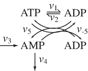
Figure 2.5: The chemical transformations involved in the distribution of high-energy phosphate bonds among adenosines.
2.3.1. Distribution of high-energy phosphate among the adenylate phosphates
In Figure 2.5 we show the skeleton structure of the transfer of high-energy phosphate bonds among the adenylates. In this figure we denote the use of ATP by \(v_1\) and the synthesis of ATP from ADP by \(v_2\), \(v_5\) and \(v_{-5}\) denote the reaction rates of adenylate kinase that distributes the high energy phosphate bonds among ATP, ADP, and AMP, through the reaction
Finally, the synthesis of AMP and its degradation is denoted by \(v_3\) and \(v_4\), respectively. The dynamic mass balance equations that describe this schema are:
The responsiveness of these reactions falls into three categories: \(v_{5, net} (=v_5 - v_{-5})\) is a fast reversible reaction, \(v_1\) and \(v_2\) have intermediate time scales, and the kinetics of \(v_3\) and \(v_4\) are slow and have large time constants associated with them. Based on this time scale decomposition, we can combine the three concentrations so that they lead to the elimination of the reactions of a particular response time category on the right hand side of (Eq. 2.13). These combinations are as follows:
First, we can eliminate all but the slow reactions by forming the sum of the adenosine phosphates.
\[\begin{equation} \frac{d}{dt}(\text{ATP} + \text{ADP} + \text{AMP}) = v_3 - v_4\ \text{(slow)} \tag{2.14} \end{equation}\]The only reaction rates that appear on the right hand side of the equation are \(v_3\) and \(v_4\), that are the slowest reactions in the system. Thus, the summation of ATP, ADP, and AMP is a pool or aggregate variable that is expected to exhibit the slowest dynamics in the system.
The second pooled variable of interest is the summation of 2ATP and ADP that represents the total number of high energy phosphate bonds found in the system at any given point in time:
\[\begin{equation} \frac{d}{dt}(2 \text{ATP} + \text{ADP}) = -v_1 + v_2\ \text{(intermediate)} \tag{2.15} \end{equation}\]This aggregate variable is only moved by the reaction rates of intermediate response times, those of \(v_1\) and \(v_2\).
The third aggregate variable we can form is the sum of the energy carrying nucleotides which are
\[\begin{equation} \frac{d}{dt}(\text{ATP} + \text{ADP}) = -v_{5, net}\ \text{(fast)} \tag{2.16} \end{equation}\]This summation will be the fastest aggregate variable in the system.
Notice that by combining the concentrations in certain ways, we define aggregate variables that may move on distinct time scales in the simple model system, and, in addition, we can interpret these variables in terms of their metabolic physiological significance. However, in general, time scale decomposition is more complex as the concentrations that influence the rate laws may move on many time scales and the arguments in the rate law functions must be pooled as well.
2.3.2. Using ratios of aggregate variables to describe metabolic physiology
We can define an aggregate variable that represents the capacity to carry high-energy phosphate bonds. That simply is the summation of \(\text{ATP} + \text{ADP} + \text{AMP}.\) This number multiplied by 2 would be the total number of high energy phosphate bonds that can be stored in this system. The second variable that we can define here would be the occupancy of that capacity, \(\textit{2ATP + ADP}\), which is simply an enumeration of how much of that capacity is occupied by high-energy phosphate bonds. Notice that the occupancy variable has a conjugate pair, which would be the vacancy variable. The ratio of these two aggregate variables forms a charge
called the energy charge, given by
which is a variable that varies between 0 and 1. This quantity is the energy charge defined by Daniel Atkinson (Atkinson, 1968). In cells, the typical numerical range for this variable when measured is 0.80-0.90.
In a similar way, one can define other redox charges. For instance, the catabolic redox charge on the NADH carrier can be defined as
which simply is the fraction of the NAD pool that is in the reduced form of NADH. It typically has a low numerical value in cells, i.e., about 0.001-0.0025, and therefore this pool is typically discharged by passing the redox potential to the electron transfer system (ETS). The anabolic redox charge
in contrast, tends to be in the range of 0.5 or higher, and thus this pool is charged and ready to drive biosynthetic reactions. Therefore, pooling variables together based on a time scale hierarchy and chemical characteristics can lead to aggregate variables that are physiologically meaningful.
In Chapter 8 we further explore these fundamental concepts of time scale hierarchy. They are then used in Parts III and IV in interpreting the dynamic states of realistic biological networks.
2.4. Time Scale Decomposition
2.4.1. Reduction in dimensionality
As illustrated by the examples given in the previous section, most biochemical reaction networks are characterized by many time constants. Typically, these time constants are of very different orders of magnitude. The hierarchy of time constants can be represented by the time axis, Figure 2.6. Fast transients are characterized by the processes at the extreme left and slow transients at the extreme right. The process time scale, i.e., the time scale of interest, can be represented by a window of observation on this time axis. Typically, we have three principal ranges of time constants of interest if we want to focus on a limited set of events taking place in a network. We can thus decompose the system response in time. To characterize network dynamics completely we would have to study all the time constants.
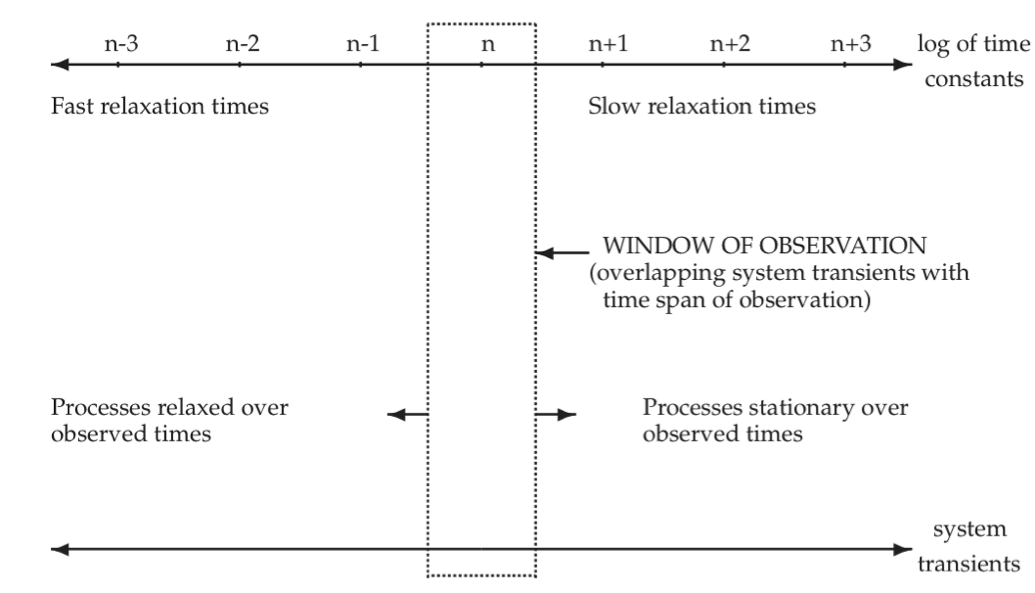
Figure 2.6: Schematic illustration of network transients that overlap with the time span of observation. n, n + 1, … represent the decadic order of time constants.
2.4.2. Three principal time constants
One can readily conceptualize this by looking at a three-dimensional linear system where the first time constant represents the fast motion, the second represents the time scale of interest, and the third is a slow motion, see Figure 2.7. The general solution to a three-dimensional linear system is
where \(\textbf{v}_i\) are the eigenvectors, \(\textbf{u}_i\) are the eigenrows, and \(\boldsymbol{\lambda}_i\) are the eigenvalues of the Jacobian matrix. The eigenvalues are negative reciprocals of time constants.
The terms that have time constants faster than the observed window can be eliminated from the dynamic description as these terms are small. However, the mechanisms which have transients slower than the observed time exhibit high “inertia” and hardly move from their initial state and can be considered constants.
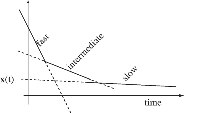
Figure 2.7: A schematic of a decay comprised of three dynamic modes with well-separated time constants.
2.4.2.1. Example: 3D motion simplifying to a 2D motion
Figure 2.8 illustrates a three-dimensional space where there is rapid motion into a slow two-dimensional subspace. The motion in the slow subspace is spanned by two “slow” eigenvectors, whereas the fast motion is in the direction of the “fast” eigenvector.
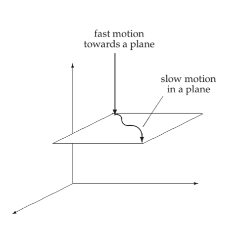
Figure 2.8: Fast motion into a two-dimensional subspace.
2.4.3. Multiple time scales
In reality there are many more than three time scales in a realistic network. In metabolic systems there are typically many time scales and a hierarchical formation of pools, Figure 2.9. The formation of such hierarchies will be discussed in Parts III and IV of the text.
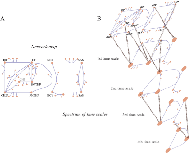
Figure 2.9: Multiple time scales in a metabolic network and the process of pool formation. This figure represents human folate metabolism. (a) A map of the folate network. (b) An illustration progressive pool formation. Beyond the first time scale pools form between CHF and CH2F; and 5MTHF, 10FTHF, SAM; and MET and SAH (these are abbreviations for the long, full names of these metabolites). DHF and THF form a pool beyond the second time scale. Beyond the third time scale CH2F/CHF join the 5MTHF/10FTHF/SAM pool. Beyond the fourth time scale HCY joins the MET/SAH pool. Ultimately, on time scales on the order of a minute and slower, interactions between the pools of folate carriers and methionine metabolites interact. Courtesy of Neema Jamshidi (Jamshidi, 2008a).
2.5. Network Structure versus Dynamics
The stoichiometric matrix represents the topological structure of the network, and this structure has significant implications with respect to what dynamic states a network can take. Its null spaces give us information about pathways and pools. It also determines the structural features of the gradient matrix. Network topology can have a dominant effect on network dynamics.
2.5.1. The null spaces of the stoichiometric matrix
Any matrix has a right and a left null space. The right null space, normally called just the null space, is defined by all vectors that give zero when post-multiplying that matrix:
The null space thus contains all the steady state flux solutions for the network. The null space can be spanned by a set of basis vectors that are pathway vectors (SB1).
The left null space is defined by all vectors that give zero when pre-multiplying that matrix:
These vectors \(\textbf{l}\) correspond to pools that are always conserved at all time scales. We will call them time invariants. Throughout the book we will look at these properties of the stoichiometric matrices that describe the networks being studied.
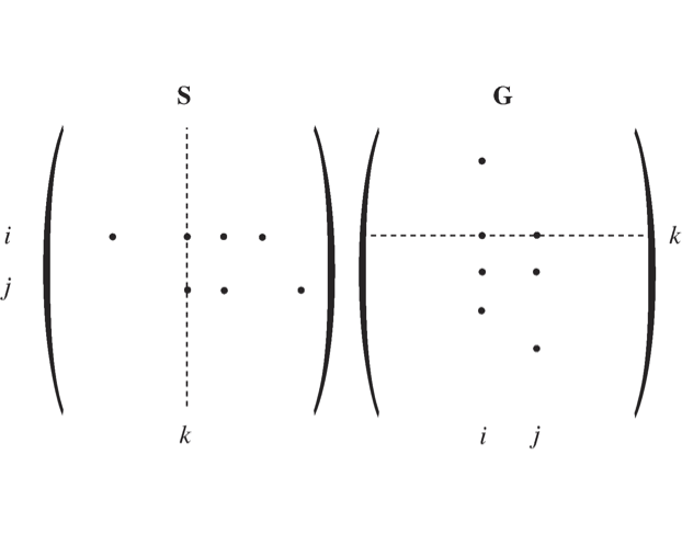
Figure 2.10: A schematic showing how the structure of \(\textbf{S}\) and \(\textbf{G}\) form matrices that have non-zero elements in the same location if one of these matrices is transposed. The columns of \(\textbf{S}\) and the rows of \(\textbf{G}\) have similar but not identical vectors in an n-dimensional space. Note that this similarity only holds once the two opposing elementary reactions have been combined into a net reaction.
2.5.2. The structure of the gradient matrix
We will now examine some of the properties of \(\textbf{G}\). If a compound \(x_i\) participates in reaction \(v_j\), then the entry \(s_{i,j}\) is non-zero. Thus, a net reaction
with a net reaction rate
generates three non-zero entries in \(\textbf{S}\): \(s_{i,j}\), \(s_{i + 1,j}\), and \(s_{i + 2,j}\). Since compounds \(x_i\), \(x_{i + 1}\), and \(x_{i + 2}\) influence reaction \(v_j\), they will also generate non-zero elements in \(\textbf{G}\), see Figure 2.10. Thus, non-zero elements generated by the reactions are:
In general, every reaction in a network is a reversible reaction. Hence we have the the following relationships between the elements of \(\textbf{S}\) and \(\textbf{G}\):
Note that for the rare cases where a reaction is effectively irreversible, an element in \(\textbf{G}\) can become very small, but in principle finite.
It can thus be seen that
in the sense that both will have non-zero elements in the same location. These elements will have opposite signs.
2.5.3. Stoichiometric autocatalysis
The fundamental structure of most catabolic pathways in a cell is such that a compound is imported into a cell and then some property stored on cofactors is transferred to the compound and the molecule is thus “charged” with this property. This charged form is then degraded into a waste product that is secreted from the cell. During that degradation process, the property that the molecule was charged with is re-extracted from the compound, often in larger quantities than was used in the initial charging of the compound. This pathway structure is the cellular equivalent of “it takes money to make money,” and its basic network structure is in Figure 2.11.
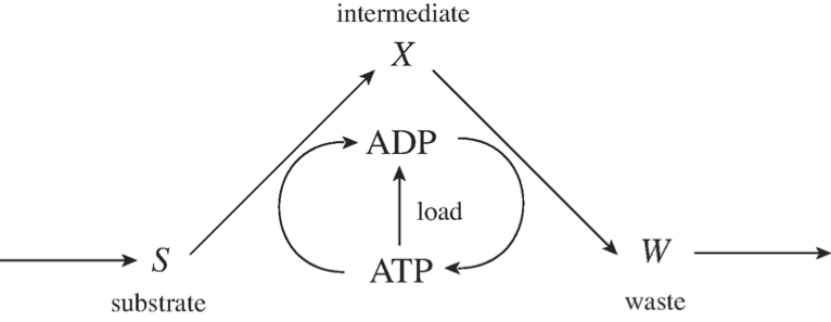
Figure 2.11: The prototypic pathway structure for degradation of a carbon substrate.
This figure illustrates the import of a substrate, \(S\), to a cell. It is charged with high-energy phosphate bonds to form an intermediate, \(X\). \(X\) is then subsequently degraded to a waste product, \(W\), that is secreted. In the degradation process, ATP is recouped in a larger quantity than was used in the charging process. This means that there is a net production of ATP in the two steps, and that difference can be used to drive various load functions on metabolism.
The consequence of this schema is basically stoichiometric autocatalysis that can lead to multiple steady states. The rate of formation of \(\text{ATP}\) from this schema as balanced by the load parameters is illustrated in Figure 2.12. This figure shows that the \(\text{ATP}\) generation is 0 if all the adenosine phosphates are in the form of \(\text{ATP}\) because there is no \(\text{ADP}\) to drive the conversion of X to W. The \(\text{ATP}\) generation is also 0 if there is no \(\text{ATP}\) available, because \(S\) cannot be charged to form \(X\). The curve in between \(\text{ATP} = 0\) and \(\text{ATP} = \text{ATP}_{max}\) will be positive. The \(\text{ATP}\) load, or use rate, will be a curve that grows with \(\text{ATP}\) concentration and is sketched here as a hyperbolic function. As shown, there are three intersections in this curve, with the upper stable steady-state being the physiological state of this system. This system can thus have multiple steady-states and this property is a consequence of the topological structure of this reaction network.
2.5.4. Network structure
The three topics discussed in this section show that the stoichiometric matrix has a dominant effect on integrated network functions and sets constraints on the dynamic states that a network can achieve. The numerical values of the elements of the gradient matrix determine which of these states are chosen.
2.6. Physico-Chemical Effects
Molecules have other physico-chemical properties besides the collision rates that are used in kinetic theory. They also have osmotic properties and are electrically charged. Both of these features influence dynamic descriptions of biochemical reaction networks.
2.6.1. The constant volume assumption
Most systems that we identify in systems biology correspond to some biological entity. Such entities may be an organelle like the nucleus or the mitochondria, or it may be the whole cell, as illustrated in Figure 2.13.
A compound, \(x_i\), internal to the system, has a mass balance on the total amount per cell. We denote this quantity with an \(M_i\). \(M_i\) is a product of the volume per cell, \(V\), and the concentration of the compound, \(x_i\), which is amount per volume
The time derivative of the amount per cell is given by:
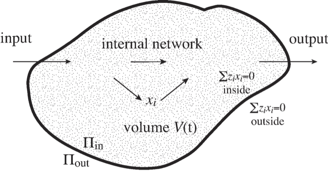
Figure 2.13: An illustration of a ‘system’ with a defined boundary, inputs and outputs, and an internal network of reactions. The \(V\) volume of the system may change over time. \(\Pi\) denotes osmotic pressure, see (Eq. 2.32).
The time change of the amount \(M_i\) per cell is thus dependent on two dynamic variables. One is \(dx_i/dt\) which is the time change in the concentration of \(x_i\), and the second is \(dV/dt\) which is the change in volume with time. The volume is typically taken to be time invariant and therefore the term \(dV/dt\) is equal to 0 and therefore results in a system that is of constant volume. In this case
This constant volume assumption (recall Table 1.2) needs to be carefully scrutinized when one builds kinetic models since volumes of cellular compartments tend to fluctuate and such fluctuations can be very important. Very few kinetic models in the current literature account for volume variation because it is mathematically challenging and numerically difficult to deal with. A few kinetic models have appeared, however, that do take volume fluctuations into account (Joshi, 1989m and Klipp, 2005).
2.6.2. Osmotic balance
Molecules come with osmotic pressure, electrical charge, and other properties, all of which impact the dynamic states of networks. For instance, in cells that do not have rigid walls, the osmotic pressure has to be balanced inside \((\Pi_{in})\) and outside \((\Pi_{out})\) of the cell (Figure 2.13), i.e.,
At first approximation, osmotic pressure is proportional to the total solute concentration,
although some compounds are more osmotically-active than others and have osmotic coefficients that are not unity. The consequences are that if a reaction takes one molecule and splits it into two, the reaction comes with an increase in osmotic pressure that will impact the total solute concentration allowable inside the cell, as it needs to be balanced relative to that outside the cell. Osmotic balance equations are algebraic equations that are often complicated and therefore are often conveniently ignored in the formulation of a kinetic model.
2.6.3. Electroneutrality
Another constraint on dynamic network models is the accounting for electrical charge. Molecules tend to be charged positively or negatively. Elementary charges cannot be separated, and therefore the total number of positive and negative charges within a compartment must balance. Any import and export in and out of a compartment of a charged species has to be counterbalanced by the equivalent number of molecules of the opposite charge crossing the membrane. Typically, bilipid membranes are impermeable to cations, but permeable to anions. For instance, the deliberate displacement of sodium and potassium by the ATP-driven sodium potassium pump is typically balanced by chloride ions migrating in and out of a cell or a compartment leading to a state of electroneutrality both inside and outside the cell. The equations that describe electroneutrality are basically a summation of the charge, \(z_i\), of a molecule multiplied by its concentration,
and such terms are summed up over all the species in a compartment. That sum has to add up to 0 to maintain electroneutrality. Since that summation includes concentrations of species, it represents an algebraic equation that is a constraint on the allowable concentration states of a network.
2.7. Summary
Time constants are key quantities in dynamic analysis. Large biochemical reaction networks typically have a broad spectrum of time constants.
Well-separated time constants lead to pooling of variables to form aggregates. Aggregate variables represent a coarse-grained (i.e., lower dimensional) view of network dynamics and can lead to physiologically meaningful variables.
Elementary reactions and mass action kinetics are the irreducible events in dynamic descriptions of networks. Elementary reactions are often combined into reaction mechanisms from which rate laws are derived using simplifying assumptions.
Network structure has an overarching effect on network dynamics. Certain physico-chemical effects can as well. Thus topological analysis is useful, and so is a careful examination of the assumptions (recall Table 1.2) that underlie the dynamic mass balances (Eq. (1.1)) for the system being modeled and simulated.
\(\tiny{\text{© B. Ø. Palsson 2011;}\ \text{This publication is in copyright.}\\ \text{Subject to statutory exception and to the provisions of relevant collective licensing agreements,}\\ \text{no reproduction of any part may take place without the written permission of Cambridge University Press.}}\)